Quantitative Finance: The Best Books to Learn It, In Order
This curriculum is designed for expert-level practitioners who already command graduate mathematics and want to achieve deep mastery of quantitative finance — from the rigorous measure-theoretic foundations of stochastic calculus, through derivatives pricing theory, to cutting-edge models and live algorithmic strategies. Each stage builds directly on the last: the mathematics unlocks the theory, the theory unlocks the models, and the models unlock the strategies.
Rigorous Stochastic Calculus Foundations
ExpertCommand measure-theoretic probability, Itô calculus, martingales, and stochastic differential equations at a research level — the mathematical bedrock for everything that follows.
▸ Study plan for this stage
Pace: 12–14 weeks, ~40–50 pages/day (with 2–3 days/week for problem sets and proofs). Karatzas (Chapters 1–5): 4 weeks; Oksendal (Chapters 1–5): 4 weeks; Merton (Chapters 1–3, selected sections): 3–4 weeks.
- Measure-theoretic probability: σ-algebras, filtrations, conditional expectation, and the Radon-Nikodym theorem as the foundation for all stochastic modeling
- Brownian motion: construction, path properties (continuity, non-differentiability), quadratic variation, and its role as the canonical continuous martingale
- Itô calculus: the Itô integral, Itô's lemma, and the chain rule for stochastic processes—the core computational tool for SDEs
- Martingales and semimartingales: martingale properties, optional stopping, Doob's inequalities, and decomposition into martingale and finite-variation parts
- Stochastic differential equations: existence and uniqueness theorems, strong vs. weak solutions, and the connection between SDEs and PDEs via Feynman-Kac
- Girsanov's theorem: change of measure and risk-neutral pricing foundations—the bridge from real-world to risk-neutral dynamics
- Stochastic exponentials and Novikov's condition: ensuring well-defined martingale densities for measure changes
- Applications to continuous-time finance: geometric Brownian motion, the Black-Scholes framework, and portfolio optimization as concrete instantiations of SDE theory
- What is the Itô integral, how does it differ from a Riemann integral, and why is the quadratic variation of Brownian motion essential to its definition?
- State and prove Itô's lemma for a general semimartingale, and apply it to derive the SDE for f(B_t) where B_t is Brownian motion and f is twice continuously differentiable.
- Define a martingale, explain the optional stopping theorem, and give an example where the theorem applies and one where it fails due to integrability conditions.
- What are the sufficient conditions for existence and uniqueness of solutions to an SDE, and how do Lipschitz and linear growth conditions ensure a strong solution?
- Explain Girsanov's theorem: how does it allow us to change the probability measure, and why is Novikov's condition necessary?
- Derive the Black-Scholes PDE from the SDE for a stock price using Itô's lemma and a self-financing portfolio argument, then connect it to the Feynman-Kac formula.
- Work through Karatzas Chapter 2 (Brownian motion): compute the quadratic variation [B, B]_t directly from the definition, verify that the sample paths are continuous but nowhere differentiable, and prove that B_t is a martingale using the definition.
- Solve 5–8 problems from Karatzas Chapter 3 (Itô integral) on computing Itô integrals explicitly (e.g., ∫₀ᵗ B_s dB_s, ∫₀ᵗ s dB_s) and verifying martingale properties.
- Apply Itô's lemma (Karatzas Chapter 4) to derive SDEs for functions of Brownian motion: (a) d(B_t²), (b) d(exp(B_t)), (c) d(sin(B_t)), and verify your results by direct computation.
- Prove the existence and uniqueness theorem for SDEs (Oksendal Chapter 5) under Lipschitz conditions; then construct a counterexample where uniqueness fails (e.g., dX_t = √|X_t| dB_t).
- Work through Oksendal Chapter 3 (Itô's formula) and Chapter 4 (Stochastic differential equations): solve 6–10 problems on solving SDEs explicitly (geometric Brownian motion, Ornstein-Uhlenbeck, etc.) and verifying solutions.
- Implement Girsanov's theorem (Oksendal Chapter 8 or Karatzas Chapter 3.5): change the measure for a geometric Brownian motion from the real-world to risk-neutral, verify Novikov's condition, and confirm that the discounted stock price becomes a martingale.
- Derive the Black-Scholes PDE from first principles using Merton Chapter 1–2: start with the SDE for S_t, construct a replicating portfolio, apply Itô's lemma, and show that the option value satisfies the PDE.
- Solve 4–6 problems from Merton Chapter 3 on continuous-time portfolio optimization: set up the Bellman equation, use Itô's lemma to derive the HJB equation, and solve for optimal consumption and investment policies.
Next up: Mastery of measure-theoretic probability, Itô calculus, and SDEs provides the rigorous mathematical machinery needed to move into advanced derivative pricing, stochastic volatility models, and portfolio theory—where you will apply these tools to real market problems and exotic instruments.

The definitive graduate-level reference for Brownian motion, martingales, and Itô integration. Reading this first establishes the rigorous probabilistic language used in every subsequent text.
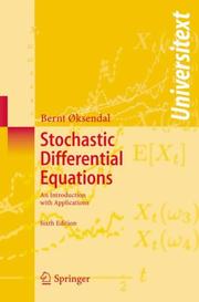
Bridges pure theory to applied SDEs with clean proofs and finance-oriented examples. Read after Karatzas to consolidate intuition and see the machinery applied concretely.

Merton's collected foundational papers, read here to see how stochastic calculus was originally wielded to derive economic results — the essential intellectual link between pure math and finance theory.
Derivatives Pricing Theory
ExpertDerive and deeply understand risk-neutral pricing, the fundamental theorems of asset pricing, and the full Black-Scholes-Merton framework and its extensions.
▸ Study plan for this stage
Pace: 8–10 weeks, ~40–50 pages/day (mix of theory and worked examples)
- Martingale theory and its role as the foundation for risk-neutral pricing under the measure-theoretic framework
- Filtrations, adapted processes, and the mathematical structure of information flow in financial markets
- Girsanov's theorem and the change of measure: how to construct and interpret the risk-neutral measure
- The fundamental theorems of asset pricing: no-arbitrage ⟺ existence of equivalent martingale measure, and completeness ⟺ uniqueness
- Stochastic differential equations (SDEs) for asset prices and the Itô lemma for computing derivatives of stochastic processes
- The Black-Scholes-Merton PDE derivation via replication and martingale methods, and closed-form solutions for European options
- Volatility smile, local volatility models, and stochastic volatility extensions (Heston model) as responses to market realities
- Numerical methods: binomial trees, finite difference schemes, and Monte Carlo simulation for pricing when closed-form solutions don't exist
- What is a martingale measure, why does it exist under no-arbitrage, and how does it enable risk-neutral pricing?
- State and explain the two fundamental theorems of asset pricing: what do no-arbitrage and market completeness imply?
- Derive the Black-Scholes-Merton PDE using both the replication argument and the martingale approach; explain why both give the same answer
- What is Girsanov's theorem, and how does it allow us to change from the physical measure to the risk-neutral measure?
- How does the Itô lemma relate to the chain rule in ordinary calculus, and why is it essential for pricing derivatives?
- Explain the volatility smile and describe at least two model extensions (local volatility, stochastic volatility) that address it
- Work through Musiela's derivation of the martingale representation theorem and verify it for a simple two-state model; then extend to continuous time
- Implement Girsanov's theorem in a discrete-time binomial model: compute the risk-neutral probabilities and verify that discounted stock prices are martingales under the new measure
- Derive the Black-Scholes formula using both PDE methods (from Hull) and martingale methods (from Musiela); reconcile the two approaches step-by-step
- Apply Itô's lemma to compute d(S²) and d(ln S) for geometric Brownian motion; verify your results against Hull's examples
- Calibrate a binomial tree (Hull) to match Black-Scholes prices for a European call; then price an American option and explain the early-exercise premium
- Implement a Monte Carlo simulation to price a European call and a barrier option; compare against analytical or binomial benchmarks and discuss convergence
- Solve a stochastic volatility problem (e.g., Heston-type) numerically using finite differences or Monte Carlo; compare implied volatility curves to the market smile
Next up: Mastery of risk-neutral pricing and the Black-Scholes framework provides the theoretical and computational foundation for the next stage, which will likely extend to interest-rate derivatives, exotic options, and multi-asset pricing—all of which rely on the same martingale and PDE machinery applied to more complex payoffs and market models.
The most mathematically complete treatment of arbitrage pricing, change of numeraire, and term-structure theory. Start here to get the full measure-theoretic pricing framework in one place.

Read after Musiela as a comprehensive applied counterpart — covers every major derivative instrument and pricing formula, grounding the abstract theory in market conventions and practical detail.
Advanced Models: Volatility, Rates, and Calibration
ExpertMaster the major model families used in practice — local vol, stochastic vol, interest-rate models — and understand how they are calibrated to market data.
▸ Study plan for this stage
Pace: 12–14 weeks, ~40–50 pages/day (mix of dense theory and worked examples; allow time for calibration exercises)
- Local volatility models: construction from the volatility surface, Dupire's formula, and forward-backward PDE connections
- Stochastic volatility fundamentals: Heston model, mean reversion, volatility clustering, and smile/skew dynamics
- Interest-rate model families: short-rate models (Vasicek, CIR), HJM framework, and multi-curve dynamics in modern markets
- Model calibration: extracting parameters from market prices, least-squares optimization, and handling bid-ask spreads
- Volatility surface parameterization: SABR, SVI, and other functional forms for practical pricing and risk management
- Numerical methods for calibration: finite-difference PDE solvers, Monte Carlo simulation, and adjoint methods for Greeks
- Cross-asset effects: correlation between rates and equity vol, basis risk, and practical hedging implications
- Model validation and limits: when each model family breaks down, parameter stability, and regime changes
- How does Dupire's formula connect the volatility surface to local volatility, and what are its practical limitations when applied to real market data?
- Explain the key differences between local volatility and stochastic volatility models in terms of smile dynamics and hedging behavior.
- What is the HJM framework, and how does it unify short-rate and forward-rate models for interest-rate pricing?
- Walk through a complete calibration workflow: how would you extract Heston parameters from S&P 500 option prices, and what optimization challenges arise?
- How do modern multi-curve interest-rate models (e.g., OIS discounting) differ from single-curve assumptions, and why does this matter for derivatives pricing?
- Describe the SABR model's parameterization and explain when it is preferable to simpler volatility surface models.
- What is volatility clustering, and how do stochastic volatility models capture it better than constant-volatility assumptions?
- How would you validate a calibrated model in practice, and what red flags suggest overfitting or parameter instability?
- Implement Dupire's formula numerically: given a discrete volatility surface (strikes and maturities), compute local volatility at grid points and verify consistency with a simple European option pricer.
- Calibrate a Heston model to real or synthetic S&P 500 option data: set up the optimization problem, choose initial parameters, and compare implied vs. model prices across strikes and maturities.
- Build a finite-difference solver for the Heston PDE and price a European call; compare results to Monte Carlo and closed-form approximations.
- Fit an SVI or SABR parameterization to a volatility smile from a single maturity; then extrapolate to neighboring maturities and assess stability.
- Calibrate a Vasicek or CIR short-rate model to historical or synthetic yield-curve data; compute zero-coupon bond prices and compare to market.
- Implement a simple HJM model with a one-factor Gaussian forward-rate process; price a swaption and verify against a short-rate model for consistency.
- Conduct a sensitivity analysis: recalibrate your chosen model (local vol, Heston, or interest-rate) on different market snapshots (e.g., before/after volatility spikes) and document parameter shifts.
- Build a Monte Carlo pricer for a Bermudan swaption or exotic equity option under your calibrated stochastic volatility or interest-rate model; compute Greeks via bumping or adjoint methods.
Next up: This stage equips you with the practical model families and calibration techniques that form the foundation for advanced topics such as XVA (CVA, DVA, FVA), machine-learning-enhanced calibration, and real-time risk management in production trading systems.

The canonical practitioner-researcher text on local and stochastic volatility models, the implied vol surface, and model calibration. Essential reading before tackling multi-factor or exotic models.

The definitive reference on short-rate, HJM, and LIBOR market models with full calibration methodology. Read after Gatheral to extend mastery from equity vol to the rates world.

Covers the state-of-the-art in variance curve models and forward-variance dynamics. Read last in this stage as it synthesizes and extends everything in Gatheral and Brigo for exotic derivatives desks.
Algorithmic Trading and Quantitative Strategies
ExpertTranslate quantitative models into systematic, executable trading strategies — covering market microstructure, signal construction, portfolio optimization, and execution.
▸ Study plan for this stage
Pace: 12–14 weeks, ~40–50 pages/day with 2–3 days/week for implementation work. Allocate: Johnson (3–4 weeks), López de Prado (4–5 weeks), Isichenko (3–4 weeks), plus 1–2 weeks for integration projects.
- Market microstructure fundamentals: order types, market impact, latency, and the mechanics of electronic exchanges that underpin algorithmic execution
- Signal construction and feature engineering: building predictive signals from market data, avoiding look-ahead bias, and proper cross-validation in time-series contexts
- Machine learning in finance: ensemble methods, backtesting frameworks, and the pitfalls of overfitting in financial data (walk-forward analysis, combinatorial purged cross-validation)
- Portfolio optimization under real constraints: transaction costs, slippage, position limits, and the gap between theoretical and implementable portfolios
- Execution algorithms: VWAP, TWAP, implementation shortfall, and how to minimize market impact and adverse selection
- Risk management in systematic strategies: Sharpe ratio, maximum drawdown, stress testing, and regime-dependent performance
- From research to production: translating backtested models into live trading systems with proper monitoring, rebalancing, and adaptation
- What is market impact, how does it scale with order size, and why is it critical to account for in algorithmic execution?
- How do you construct a robust trading signal that avoids look-ahead bias and overfitting, and what cross-validation methods are appropriate for time-series data?
- What are the key differences between VWAP and TWAP algorithms, and when would you choose one over the other?
- How do transaction costs, slippage, and market impact affect the feasibility of a strategy developed in backtesting, and how do you bridge this gap?
- What is the purpose of walk-forward analysis and combinatorial purged cross-validation, and why are standard ML cross-validation techniques insufficient for financial data?
- How do you construct a mean-variance efficient portfolio that accounts for real-world constraints (position limits, transaction costs, liquidity), and what are the failure modes of classical Markowitz optimization?
- What metrics and monitoring systems would you implement to detect when a live trading strategy has degraded or entered a regime shift?
- Implement a basic market impact model (linear or square-root law) and calculate the true cost of executing a 10-day VWAP algorithm on a real stock, comparing theoretical vs. realized execution cost.
- Build a feature engineering pipeline for a simple mean-reversion signal: compute rolling z-scores, test for look-ahead bias, and validate using walk-forward analysis on 5 years of daily data.
- Backtest a two-asset momentum strategy with realistic transaction costs and slippage; compare the Sharpe ratio before and after costs, and identify the breakeven trade frequency.
- Implement a combinatorial purged cross-validation framework on a classification problem (e.g., predicting next-day direction) and compare results to standard k-fold cross-validation to quantify overfitting.
- Design and code a simple portfolio optimizer that incorporates position limits, minimum position size, and transaction costs; compare the optimized portfolio to an unconstrained Markowitz solution.
- Simulate a live execution scenario: given a target portfolio and current holdings, design a rebalancing algorithm that minimizes market impact while respecting liquidity constraints.
- Conduct a regime analysis on a strategy: identify periods of outperformance and underperformance, hypothesize regime drivers (volatility, correlation, liquidity), and test whether a regime-switching model improves Sharpe ratio.
- Build a monitoring dashboard for a live strategy: track daily P&L, Sharpe ratio (rolling 60-day), maximum drawdown, turnover, and slippage; set alerts for degradation thresholds.
Next up: This stage equips you with the end-to-end toolkit to design, validate, and deploy systematic trading strategies; the next stage will deepen specialization in either advanced risk modeling, high-frequency trading mechanics, or alternative data and alternative alpha sources.

The most thorough technical treatment of market microstructure, order types, and execution algorithms. Read first in this stage to understand the market mechanics that constrain every live strategy.

Provides a rigorous, research-grade framework for building ML-driven quantitative strategies — feature engineering, backtesting pitfalls, and meta-labeling. Read after Johnson so execution realities inform model design.

A modern, practitioner-written synthesis of alpha research, factor models, and portfolio construction. Caps the curriculum by showing how signals, models, and execution combine into a full systematic investment process.
Discussion
Keep reading
Paths that share books, cover the same subject, or open a related topic.