Financial Risk Management: The Best Books, In Order
This curriculum is designed for expert-level practitioners who already command quantitative finance fundamentals and want to achieve mastery across the full spectrum of financial risk management — market, credit, and operational risk, Value at Risk, and hedging. The four stages move from the canonical theoretical frameworks through rigorous quantitative modeling, into credit and operational risk specialization, and finally into advanced hedging and integrated enterprise-level risk strategy. Each book is sequenced so that its vocabulary and models are prerequisites for the next.
Canonical Foundations & VaR Framework
ExpertEstablish a rigorous, unified mental model of financial risk — market risk taxonomy, the full Value at Risk framework (parametric, historical, Monte Carlo), and its known limitations — so every subsequent book can be read critically and deeply.
▸ Study plan for this stage
Pace: 8–10 weeks, ~40–50 pages/day (Jorion first: 4–5 weeks; Hull second: 4–5 weeks). Allocate 1–2 days per major section for synthesis and exercises.
- VaR as a unified risk metric: definition, interpretation, and why it became the industry standard despite its limitations
- The three VaR methodologies (parametric/delta-normal, historical simulation, Monte Carlo) — mathematical foundations, assumptions, computational trade-offs, and when each is appropriate
- Market risk taxonomy: equity, fixed-income, FX, and commodity risk drivers; correlation and tail dependence; stress testing vs. VaR
- The mathematics of normal distributions, quantiles, and confidence intervals in risk measurement; why normality assumptions fail in practice
- Backtesting and model validation: how to assess whether a VaR model is fit for purpose; exceptions, traffic lights, and regulatory frameworks
- Limitations and criticisms of VaR: tail risk blindness, non-subadditivity, procyclicality, and the 2008 crisis lessons
- Expected Shortfall (CVaR) and coherent risk measures as alternatives to VaR
- Regulatory context: Basel III/IV capital requirements, internal models approach, and how VaR feeds into risk governance
- Explain the mathematical definition of Value at Risk at a 95% confidence level over a 1-day horizon. Why is the choice of confidence level and time horizon not neutral?
- Compare and contrast the parametric (delta-normal), historical simulation, and Monte Carlo VaR approaches. Under what market conditions would each method fail or excel?
- What are the key assumptions underlying the parametric VaR model, and how do violations of these assumptions (non-normality, fat tails, regime shifts) affect model reliability?
- Describe the backtesting framework for VaR models. What does it mean when a VaR model experiences more exceptions than expected, and what are the regulatory consequences?
- What is Expected Shortfall (CVaR), and how does it address the main limitations of VaR? Why hasn't it completely replaced VaR in practice?
- How do correlation assumptions and tail dependence affect multi-asset VaR calculations? What happened to correlation estimates during the 2008 financial crisis?
- Explain the relationship between VaR, stress testing, and scenario analysis in a comprehensive risk framework. Why is VaR alone insufficient for risk governance?
- Implement a parametric (delta-normal) VaR calculation for a single equity position using 1 year of daily returns; compute 1-day VaR at 95% and 99% confidence levels; interpret the results.
- Implement a historical simulation VaR for the same position using the same data; compare results to parametric VaR and explain differences.
- Build a simple Monte Carlo VaR model: simulate 10,000 price paths for an equity index using geometric Brownian motion; compute 1-day VaR at 95% confidence; vary volatility assumptions and observe sensitivity.
- Backtest a parametric VaR model on real equity data (e.g., S&P 500 daily returns over 2–3 years): count exceptions, compute the exception ratio, and assess whether the model passes regulatory traffic-light tests.
- Calculate VaR for a two-asset portfolio (e.g., stocks + bonds); vary correlation assumptions from 0.3 to 0.8 and observe how portfolio VaR changes; discuss why correlation is a critical input.
- Compute Expected Shortfall (average loss beyond VaR) for a position and compare it to the VaR figure; explain why ES is more conservative and what it tells you about tail risk.
- Design a stress scenario (e.g., 2008-style equity crash + credit spread widening) and calculate portfolio losses under that scenario; compare to 1-day VaR and discuss why stress testing complements VaR.
Next up: This stage equips you with a critical, mathematically grounded understanding of VaR and its limitations, enabling the next stage to explore advanced risk models (incremental VaR, component VaR, risk attribution), operational and credit risk measurement, and integrated enterprise risk frameworks without treating VaR as gospel.
The definitive reference on VaR: covers all three estimation methodologies, backtesting, stress testing, and regulatory context. Reading this first sets the precise technical language used across the entire field.

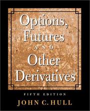
Bridges VaR theory to the institutional reality of banks and asset managers, covering market, credit, and operational risk under Basel accords — providing the regulatory scaffolding needed for all later stages.
Quantitative Market Risk & Volatility Modeling
ExpertMaster the quantitative machinery behind market risk: volatility models (GARCH, stochastic vol), extreme value theory, copulas, and coherent risk measures such as Expected Shortfall — moving well beyond VaR's limitations.
▸ Study plan for this stage
Pace: 12–14 weeks, ~40–50 pages/day (with 2–3 days/week for exercises and problem sets)
- Stochastic volatility models (GARCH, EWMA, SV) and their estimation from market data
- Extreme Value Theory (EVT): tail behavior, generalized Pareto distribution, and threshold exceedances
- Copulas: dependence structures, Gaussian/Clayton/Archimedean families, and tail dependence
- Coherent risk measures: Expected Shortfall (ES/CVaR), axioms of coherence, and advantages over VaR
- Value-at-Risk (VaR) computation: parametric, historical simulation, and Monte Carlo methods
- Backtesting and stress testing frameworks for market risk models
- Greeks and their role in derivatives pricing and risk hedging
- Correlation and covariance matrix estimation under non-normal distributions
- What are the key differences between GARCH and stochastic volatility models, and when would you choose one over the other for forecasting market risk?
- Explain how Extreme Value Theory improves upon standard normal-assumption VaR models, particularly in capturing tail risk.
- How do copulas capture dependence structures between assets, and why is tail dependence critical for portfolio risk management?
- What are the four axioms of coherent risk measures, and why does Expected Shortfall satisfy them while VaR does not?
- Walk through the calculation of VaR using parametric, historical simulation, and Monte Carlo methods—what are the trade-offs?
- How would you design a backtesting framework to validate a market risk model, and what metrics would you use?
- Implement a GARCH(1,1) model in Python or R using daily equity returns; estimate parameters via maximum likelihood and forecast 10-day volatility.
- Fit a generalized Pareto distribution to the tail of a financial return series (using threshold exceedance data) and compare EVT-based VaR to normal-assumption VaR.
- Construct a correlation matrix from multivariate returns and fit a Gaussian copula; simulate correlated asset returns and compare to historical dependence.
- Calculate VaR and Expected Shortfall (ES) for a portfolio using parametric, historical simulation, and Monte Carlo methods; document assumptions and compare results.
- Perform a backtesting analysis on a VaR model using a rolling window; compute traffic light violations and independence tests (Kupiec POF, Christoffersen).
- Price a European call option using Black–Scholes and compute all Greeks (delta, gamma, vega, theta, rho); perform a sensitivity analysis on volatility changes.
- Build a stress test scenario for a portfolio: define shocks to volatility, correlation, and tail events; measure portfolio loss under each scenario.
- Estimate a stochastic volatility model (e.g., Heston) and compare option pricing under SV vs. constant volatility; discuss the volatility smile.
Next up: This stage equips you with the quantitative foundation to model and measure market risk under realistic (non-normal, tail-heavy) conditions; the next stage will apply these tools to portfolio optimization, credit risk, and operational risk, integrating them into a comprehensive enterprise risk framework.
Provides the rigorous derivatives-pricing and measure-theory backbone — essential for understanding how market risk models are actually built and where they break down.
The graduate-level bible for market risk quants: covers coherent risk measures, EVT, copulas, and multivariate dependence — the exact toolkit needed to go beyond VaR and into ES and tail-risk modeling.
Read here (not earlier) to consolidate Greeks, volatility surfaces, and dynamic hedging mechanics that underpin market risk sensitivity analysis and hedging strategy in later stages.
Credit Risk & Operational Risk
ExpertDevelop deep expertise in credit risk modeling (structural, reduced-form, portfolio credit risk, CDOs) and operational risk measurement (LDA, scenario analysis, Basel AMA), completing the Basel risk-type triad.
▸ Study plan for this stage
Pace: 12–14 weeks, ~40–50 pages/day (mix of theory-dense sections and technical chapters; allow 2–3 days per major model framework)
- Structural credit risk models (Merton framework): how firm value dynamics and leverage determine default probability and credit spreads
- Reduced-form (intensity-based) models: hazard rates, survival probabilities, and calibration to market prices without firm-value assumptions
- Portfolio credit risk: correlation structures, loss distributions, and the role of systematic vs. idiosyncratic risk in portfolio default losses
- Collateralized Debt Obligations (CDOs): tranching mechanics, subordination, and how credit enhancement redistributes risk across investor classes
- Loss Distribution Approach (LDA) for operational risk: frequency-severity modeling, Monte Carlo simulation, and tail risk quantification
- Scenario analysis and expert judgment in operational risk: complementing statistical models with forward-looking stress scenarios
- Basel AMA (Advanced Measurement Approach): regulatory framework integrating LDA, scenario analysis, and business-line risk capital allocation
- Model validation and backtesting: assessing credit and operational risk model performance against realized outcomes
- Explain the Merton structural model: how does firm value evolution determine default time, and what are its key limitations in practice?
- Compare structural and reduced-form credit risk models: when is each approach most appropriate, and how do they differ in their treatment of default triggers?
- Describe the mechanics of CDO tranching: how do subordination and credit enhancement affect the risk and return profile of each tranche, and what role does correlation play?
- What is the Loss Distribution Approach (LDA) for operational risk, and how do frequency and severity distributions combine to produce a tail risk estimate?
- How does scenario analysis complement statistical operational risk models, and what are the challenges in integrating expert judgment with quantitative LDA?
- Outline the Basel AMA framework: what are its three pillars, and how do credit and operational risk capital charges fit into overall regulatory capital requirements?
- Implement a Merton structural model in a spreadsheet or Python: calibrate firm value and volatility to market equity data, compute default probability, and compare to CDS spreads for a real company
- Build a reduced-form intensity model: estimate hazard rates from historical default data or market CDS quotes, compute survival curves, and price a corporate bond under different recovery assumptions
- Construct a simple two-asset portfolio credit risk model: specify correlation, simulate joint defaults, and compute portfolio loss distribution and Value-at-Risk (VaR) at 99.9% confidence
- Analyze a real CDO structure: obtain a prospectus or synthetic example, trace cash flows through tranches, compute subordination levels, and explain how correlation stress affects tranche losses
- Develop an LDA operational risk model: collect or simulate frequency and severity data for a business line, fit distributions (Poisson/negative binomial for frequency, lognormal/Pareto for severity), run Monte Carlo simulation, and estimate capital at 99.9% confidence
- Conduct a scenario analysis exercise: define 3–4 forward-looking operational risk scenarios (e.g., IT system failure, fraud, regulatory breach), estimate loss ranges, and compare to LDA tail estimates
Next up: This stage completes the Basel risk-type triad (market, credit, operational) and establishes the quantitative and regulatory foundations needed to advance into integrated risk management, stress testing, and enterprise risk frameworks in the next stage.
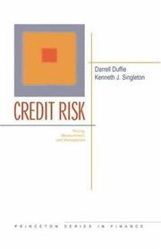
The authoritative academic treatment of structural and reduced-form credit models, credit derivatives pricing, and portfolio credit risk — the essential starting point for serious credit risk work.

Complements Duffie with a practitioner-oriented view of credit scoring, CreditMetrics, KMV, and regulatory capital — bridging theory to bank credit portfolio management.

One of the few rigorous, book-length treatments of operational risk measurement: covers loss distribution approaches, EVT applied to op risk, scenario analysis, and Basel II/III AMA requirements.
Advanced Hedging & Integrated Risk Strategy
ExpertSynthesize everything into sophisticated, real-world hedging strategies — dynamic delta/gamma/vega hedging, interest rate and FX risk hedging, and enterprise-wide risk management — thinking like a chief risk officer.
▸ Study plan for this stage
Pace: 12–14 weeks, ~40–50 pages/day (with 2–3 days/week for exercises and synthesis)
- Dynamic delta hedging: continuous rebalancing, gamma risk, and the cost of hedging in discrete time and real market conditions
- Gamma and vega management: understanding convexity, volatility exposure, and the Greeks as hedging tools across market regimes
- Volatility surface construction and interpretation: term structure, skew, smile, and how to model and trade volatility risk
- Interest rate and FX hedging: applying Greeks and volatility concepts to multi-currency and fixed-income portfolios
- Bleed and slippage: transaction costs, bid-ask spreads, and gap risk in real-world hedging implementation
- Enterprise-wide risk aggregation: correlations, tail risk, and stress testing across asset classes and business units
- Behavioral and philosophical foundations: uncertainty, probability, and the evolution of risk thinking from Bernstein's historical perspective
- How does gamma risk emerge in delta-hedged portfolios, and why does continuous rebalancing in discrete time create a cost that must be managed?
- What is the volatility surface, how does it differ from a flat volatility assumption, and how do skew and term structure inform hedging decisions?
- How would you design a dynamic hedging program for a large options book that accounts for transaction costs, liquidity constraints, and gap risk?
- What are the key differences between hedging single-currency equity volatility versus multi-currency FX and interest rate risk, and how do correlations complicate enterprise risk?
- How do you construct and stress-test a firm-wide risk dashboard that aggregates delta, gamma, vega, and correlation risk across multiple business units?
- What historical lessons from the evolution of probability and risk thinking (Bernstein) inform your approach to tail risk and model uncertainty in modern hedging?
- Build a dynamic delta-hedging simulator in Excel or Python: track a long call position, rebalance daily, and measure realized P&L versus theoretical gamma bleed and transaction costs over 3–6 months of historical data.
- Extract and visualize a volatility surface from real or simulated option prices; identify skew, term structure, and smile effects; explain how each would affect your hedging ratios.
- Design a hedging policy for a 100M USD equity derivatives book: specify delta, gamma, and vega limits; document rebalancing triggers; estimate monthly hedging costs under normal and stressed market conditions.
- Construct a multi-asset risk report: aggregate delta, gamma, vega, and correlation risk across equities, FX, and fixed income; identify concentrations and propose hedges.
- Perform a stress test on a hedged portfolio: apply historical scenarios (2008 crisis, COVID, vol spike) and measure P&L impact; identify basis risk and correlation breakdowns.
- Write a 2–3 page memo as a chief risk officer: synthesize Taleb's hedging philosophy, Gatheral's volatility insights, and Bernstein's risk history to justify a firm's hedging strategy to the board.
Next up: This stage equips you with the technical and strategic mastery to implement enterprise-wide hedging and risk governance; the next stage will deepen specialized domains (e.g., credit risk modeling, operational risk frameworks, or regulatory capital optimization) or move to real-time portfolio management and algorithmic execution.
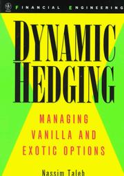
An unmatched practitioner deep-dive into the real mechanics of hedging options books: path dependency, discrete rebalancing, and the fragility of model-based hedges — essential reading before managing any trading book.
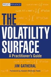
Provides the advanced market-implied volatility modeling needed to hedge exotic and structured products correctly, connecting stochastic vol models to live market data.

Read last as a capstone: reframes the entire history and philosophy of risk measurement, sharpening the expert's judgment about where quantitative models are trustworthy and where human judgment must prevail.
Discussion
Keep reading
Paths that share books, cover the same subject, or open a related topic.