The Best Books to Learn Stochastic Processes
This curriculum is designed for expert-level learners who already have strong foundations in probability and analysis, and want to achieve deep mastery of stochastic processes. The path moves from rigorous measure-theoretic foundations through the core pillars — Markov chains, Poisson processes, and Brownian motion — and culminates in advanced stochastic calculus and random dynamics, building both theoretical depth and analytical power at each stage.
Measure-Theoretic Probability & Process Foundations
ExpertSolidify the rigorous probabilistic infrastructure — σ-algebras, filtrations, martingales, and convergence theorems — that underpins all modern stochastic process theory.
▸ Study plan for this stage
Pace: 8–10 weeks, ~40–50 pages/day (Williams ~300 pages in 6–7 weeks; Durrett ~500 pages in 3–4 weeks, with overlap on core topics)
- σ-algebras, measurable spaces, and the Borel σ-algebra as the foundation for rigorous probability
- Probability measures, Lebesgue integration, and the Radon–Nikodym theorem for measure-theoretic probability
- Conditional expectation as a projection operator and its properties (tower law, independence)
- Filtrations, adapted processes, and stopping times as the temporal structure of stochastic processes
- Martingales, submartingales, supermartingales, and their fundamental properties (optional stopping, Doob's inequality)
- Convergence theorems: dominated convergence, monotone convergence, Fatou's lemma, and martingale convergence
- Uniform integrability and L¹ convergence of martingales
- Quadratic variation and the Itô isometry as bridges to continuous-time processes
- What is a σ-algebra, and why is it the natural domain for a probability measure? How does the Borel σ-algebra arise on ℝ?
- Define conditional expectation rigorously using the Radon–Nikodym theorem. Why is it a projection, and what does the tower law tell us?
- What is a filtration, and how do adapted processes and stopping times formalize the notion of information flow in time?
- State and explain the martingale convergence theorem. Under what conditions does a martingale converge almost surely or in L¹?
- What is Doob's inequality, and how does it control the maximum of a martingale? Why is uniform integrability essential for L¹ convergence?
- How do the dominated convergence theorem and monotone convergence theorem relate to martingale theory, and when should each be applied?
- Verify that a collection of sets forms a σ-algebra by checking closure under countable unions and complements; construct σ(𝒜) for a given collection 𝒜.
- Compute conditional expectations E[X | ℱ] for concrete random variables and filtrations; verify the tower law and independence properties.
- Work through Williams' martingale examples (simple random walk, Pólya urns, branching processes) and verify the martingale property directly.
- Apply Doob's inequality to bound P(max_{n≤N} M_n ≥ a) for a martingale (M_n); compare with Markov's inequality.
- Prove that a bounded martingale converges almost surely using the upcrossing lemma (Williams); verify L¹ convergence when uniform integrability holds.
- Construct examples where martingales fail to converge in L¹ despite a.s. convergence; identify the failure of uniform integrability.
Next up: This stage equips you with the rigorous measure-theoretic language and martingale calculus needed to define and analyze continuous-time stochastic processes (Brownian motion, Itô integrals, SDEs) and to prove convergence and invariance principles that govern their long-term behavior.

A beautifully concise yet rigorous treatment of measure-theoretic probability and martingale theory. Reading this first ensures the expert learner has the exact language and tools (conditional expectation, stopping times, optional stopping) needed for every subsequent topic.

The canonical graduate reference for measure-theoretic probability in the US tradition. Its chapters on martingales, ergodic theory, and Markov chains serve as a dense but authoritative bridge into the deeper process theory ahead.
Markov Chains — Discrete and Continuous Time
ExpertAchieve deep mastery of Markov chain theory: classification of states, stationary distributions, mixing times, reversibility, and the generator formalism for continuous-time chains.
▸ Study plan for this stage
Pace: 8–10 weeks, ~40–50 pages/day with 2–3 days/week for problem-solving and reflection
- State classification (transient, recurrent, periodic, aperiodic) and their implications for long-run behavior
- Stationary distributions: existence, uniqueness, and convergence to stationarity
- Mixing time and convergence rates: total variation distance, coupling, and spectral gap bounds
- Reversibility and detailed balance: conditions for reversible chains and their role in MCMC
- Generator matrix formalism for continuous-time Markov chains and the relationship to discrete-time chains
- Fundamental matrix and hitting times: computing expected return times and absorption probabilities
- Coupling methods as a tool for proving convergence and bounding mixing times
- Applications to Markov Chain Monte Carlo (MCMC): Metropolis–Hastings and Gibbs sampling
- How do you classify the states of a Markov chain (transient vs. recurrent, periodic vs. aperiodic), and what does each classification tell you about the chain's long-run behavior?
- Under what conditions does a finite-state Markov chain have a unique stationary distribution, and how do you compute it?
- What is mixing time, how is it formally defined using total variation distance, and what techniques (spectral gap, coupling) can bound it?
- What is reversibility and detailed balance? Why are these concepts important for MCMC algorithms?
- How do you construct and interpret the generator matrix for a continuous-time Markov chain, and what is the relationship between its eigenvalues and convergence rates?
- How do you use the fundamental matrix to compute hitting times, expected return times, and absorption probabilities?
- Classify all states in 3–4 concrete Markov chains (e.g., random walks on graphs, birth–death processes) as transient/recurrent and periodic/aperiodic; verify your classifications by computing the transition matrix powers
- For a 3×3 or 4×4 transition matrix, compute the stationary distribution by solving πP = π and verify convergence numerically by iterating the chain
- Implement a coupling argument to prove convergence for a simple chain (e.g., lazy random walk on a cycle); compute the coupling time and compare to the theoretical mixing time bound
- Write out the detailed balance equations for a reversible chain and verify that they hold; then construct a non-reversible chain and show detailed balance fails
- For a continuous-time chain, write down the generator matrix Q, compute its eigenvalues and eigenvectors, and use them to find the transition probability matrix P(t) = e^{Qt}
- Compute the fundamental matrix N = (I − Q)^{−1} for an absorbing chain and use it to find hitting times and absorption probabilities; verify results via simulation
Next up: Mastery of Markov chain theory—especially mixing times, reversibility, and the generator formalism—provides the theoretical foundation for advanced topics such as large deviations, stochastic differential equations, and applications to statistical mechanics and machine learning.

Deepens the theory with a modern focus on quantitative convergence, coupling arguments, and spectral methods. Essential for understanding the dynamical and algorithmic sides of Markov chain behavior.
Poisson Processes & General Jump Processes
ExpertUnderstand Poisson processes from first principles through to compound, spatial, and marked variants, and connect them to the broader theory of Lévy processes and random measures.
▸ Study plan for this stage
Pace: 8–10 weeks, ~40–50 pages/day (Kingman: 3–4 weeks; Sato: 5–6 weeks)
- Poisson process as a point process: definition via inter-arrival times, counting process characterization, and the memoryless property
- Intensity measure and rate parameter: connection between local behavior and global structure of Poisson processes
- Compound Poisson processes: superposition of i.i.d. jumps at Poisson times, and their role as building blocks for more complex processes
- Marked and spatial Poisson processes: extension to multi-dimensional and colored point patterns, with applications to random measures
- Lévy processes: infinite divisibility, characteristic exponents, and the Lévy–Khintchine representation
- Jump decomposition and Lévy measures: how Poisson processes and compound Poisson processes arise as components of general Lévy processes
- Infinitely divisible distributions: characterization via Lévy–Khintchine formula and connection to Lévy processes
- Random measures and point process theory: measure-theoretic foundations linking Poisson processes to general jump processes
- What is the relationship between the inter-arrival time distribution and the counting process characterization of a Poisson process, and why does the memoryless property unify them?
- How do compound Poisson processes generalize simple Poisson processes, and what role do they play in decomposing Lévy processes?
- State and explain the Lévy–Khintchine representation formula; what does each component (drift, Brownian, jump) represent?
- What is a Lévy measure, and how does it encode the jump behavior of a Lévy process? How does it relate to Poisson random measures?
- How are marked and spatial Poisson processes constructed, and what additional structure do they add beyond the standard Poisson process?
- Explain the connection between infinite divisibility and Lévy processes: why must every Lévy process have an infinitely divisible distribution at each fixed time?
- Derive the Poisson distribution from the axioms of a Poisson process (stationarity, independence, orderliness); verify that P(N(t) = k) = (λt)^k e^(−λt) / k! for a rate-λ process.
- Construct a compound Poisson process with exponentially distributed jumps; simulate sample paths and compute the mean and variance of the process at time t.
- Given a Lévy process with a specified Lévy measure ν, identify the jump component (compound Poisson part) and the continuous component; sketch the corresponding Lévy–Khintchine exponent.
- Work through Kingman's treatment of spatial Poisson processes: construct a marked Poisson process on ℝ² with intensity measure λ(dx) and mark distribution μ(dm); compute the probability that a randomly chosen point has a mark in a given set.
- Prove that if X and Y are independent infinitely divisible random variables, then X + Y is infinitely divisible; relate this to the convolution property of Lévy processes.
- For a given infinitely divisible distribution (e.g., stable distribution, gamma distribution), extract the Lévy–Khintchine parameters (a, σ², ν) from Sato's formula and interpret them in terms of process behavior.
Next up: This stage establishes Poisson and Lévy processes as the foundational building blocks of jump-type stochastic processes, positioning you to study more specialized topics such as branching processes, continuous-time Markov chains, or applications to mathematical finance and queueing theory.

The definitive monograph on Poisson processes by one of the field's masters. Kingman's elegant axiomatic approach and treatment of spatial and marked processes provides depth that no textbook chapter can match.

Places the Poisson process within the grand unified framework of Lévy processes. Reading this after Kingman reveals the deep structural reasons behind jump process behavior and prepares the reader for stochastic calculus with jumps.
Brownian Motion & Stochastic Calculus
ExpertMaster the construction and path properties of Brownian motion, the Itô integral, stochastic differential equations, and Girsanov's theorem — the analytical core of continuous-time stochastic processes.
▸ Study plan for this stage
Pace: 12–14 weeks, ~40–50 pages/day with 2–3 days/week dedicated to problem sets and computational practice
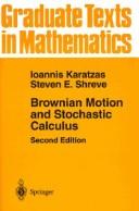
- Construction of Brownian motion via Donsker's invariance principle and the Wiener measure on path space (Mörters Ch. 1–2)
- Path properties: nowhere differentiability, quadratic variation, and the Hölder exponent of Brownian paths (Mörters Ch. 3–4)
- The Itô integral: definition via simple processes, isometry, and the fundamental difference from Riemann–Stieltjes integration (Oksendal Ch. 3)
- Itô's lemma and its application to computing differentials of functions of Brownian motion (Oksendal Ch. 4)
- Stochastic differential equations: existence, uniqueness, and strong solutions under Lipschitz conditions (Oksendal Ch. 5)
- Girsanov's theorem: change of measure and the relationship between drift and martingale properties (Oksendal Ch. 8)
- Martingale properties of Brownian motion and continuous local martingales (Revuz Ch. 1–2)
- Quadratic covariation and the bracket process in the context of semimartingales (Revuz Ch. 2–3)
- How is Brownian motion constructed via Donsker's theorem, and what does the Wiener measure represent?
- Why are Brownian paths almost surely nowhere differentiable, and what is the significance of quadratic variation?
- What is the Itô integral, how does it differ from pathwise Riemann–Stieltjes integration, and why is the Itô isometry essential?
- State and prove Itô's lemma; apply it to compute d(B_t^2) and d(e^{B_t})
- Under what conditions do stochastic differential equations have unique strong solutions, and what role does the Lipschitz condition play?
- Explain Girsanov's theorem: how does it relate the drift of an SDE to martingale properties under a change of measure?
- Verify Donsker's invariance principle numerically: simulate random walks and compare their distributions to Brownian motion at different time scales
- Compute the quadratic variation [B, B]_T = T by partitioning [0, T] and summing squared increments; observe convergence as mesh size decreases
- Construct the Itô integral ∫₀ᵗ B_s dB_s using the definition for simple processes; verify the Itô isometry E[(∫₀ᵗ B_s dB_s)²] = E[∫₀ᵗ B_s² ds]
- Apply Itô's lemma to derive: d(B_t²) = 2B_t dB_t + dt, and d(e^{B_t}) = e^{B_t}(dB_t + ½dt); verify by simulation
- Solve the geometric Brownian motion SDE dX_t = μX_t dt + σX_t dB_t explicitly; verify uniqueness via Lipschitz continuity
- Implement Girsanov's theorem: given an SDE with drift μ, construct the Radon–Nikodym derivative and verify that the drift-adjusted process is a martingale under the new measure
Next up: Mastery of Brownian motion, the Itô calculus, and Girsanov's theorem provides the technical foundation to study applications in mathematical finance (option pricing, portfolio optimization), filtering theory, and the deeper structure of general semimartingales and stochastic integration for jump processes.

A modern, rigorous, and beautifully written account of Brownian motion's construction and fine path properties (Hausdorff dimension, law of the iterated logarithm, local times). Reading this before Itô calculus builds essential geometric and analytic intuition.
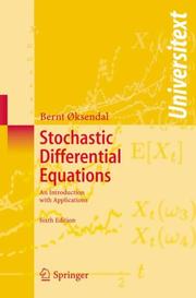
The most widely used introduction to Itô calculus and SDEs, striking the right balance between rigor and accessibility for an expert reader. Covers Itô's formula, the Feynman–Kac formula, and applications to filtering and finance.
The authoritative and exhaustive reference on continuous-time martingales, stochastic integration, and Brownian motion. After Øksendal, this book fills every theoretical gap and is the standard citation for deep results in the field.
Advanced Random Dynamics & Ergodic Theory
ExpertSynthesize everything into the study of long-run random dynamics: ergodic theory for stochastic systems, interacting particle systems, and the modern theory of stochastic processes on manifolds and in infinite dimensions.
▸ Study plan for this stage
Pace: 12–14 weeks, ~40–50 pages/day (Liggett first: 6–7 weeks; Petersen second: 6–7 weeks). Allocate 2–3 days per major topic for integration and exercises.
- Interacting particle systems as Markov processes: construction, generators, and invariant measures on infinite-dimensional state spaces
- Ergodic theory fundamentals: ergodicity, mixing, and the ergodic theorem for measure-preserving transformations
- Stationary distributions and long-run behavior: existence, uniqueness, and convergence to equilibrium in particle systems
- Duality and coupling methods: powerful tools for analyzing particle system dynamics and proving ergodic properties
- Infinite-dimensional dynamics: how ergodic theory extends to stochastic systems on function spaces and manifolds
- Interplay between microscopic interactions and macroscopic observables: how local rules generate global ergodic behavior
- Invariant measures and their characterization: the role of detailed balance, reversibility, and symmetry in stochastic systems
- What is an interacting particle system, and how is its generator constructed from local transition rates? How does this differ from finite-state Markov chains?
- State and prove the ergodic theorem. What does it mean for a measure-preserving transformation to be ergodic, and why does this imply time averages equal space averages?
- Describe the relationship between invariant measures and long-run behavior in particle systems. Under what conditions is the invariant measure unique?
- What are duality and coupling, and how do they simplify the analysis of interacting particle systems? Give a concrete example from Liggett.
- How does ergodic theory apply to infinite-dimensional stochastic systems? What additional technical challenges arise compared to finite-dimensional dynamics?
- Explain the connection between detailed balance (reversibility) and the existence of stationary distributions in particle systems.
- Work through Liggett's construction of the contact process and voter model: verify the generator, identify invariant measures, and sketch a proof that they are ergodic.
- Prove the ergodic theorem for a simple example (e.g., irrational rotation on the circle or a finite-state Markov chain) and compute time and space averages explicitly.
- Implement a Monte Carlo simulation of a simple interacting particle system (e.g., exclusion process or contact process on a finite lattice) and verify convergence to the invariant measure numerically.
- Use coupling to prove that two copies of a particle system coalesce (or diverge) appropriately; connect this to ergodicity and mixing.
- Characterize the invariant measures for a specific particle system from Liggett (e.g., the symmetric exclusion process) using detailed balance or a variational principle.
- Analyze the ergodic properties of a stochastic differential equation or Langevin dynamics on a manifold: verify the invariant measure and mixing time.
Next up: This stage equips you with the theoretical framework to study long-run behavior of complex stochastic systems; the next stage will apply these tools to modern topics such as large deviations, metastability, and stochastic partial differential equations, where ergodic theory and particle system intuition become essential.

The definitive text on infinite systems of interacting Markov processes, including contact processes, voter models, and exclusion processes. Brings together Markov chain, Poisson, and martingale theory in a rich dynamical setting.

Provides the measure-theoretic ergodic foundations — ergodic theorems, entropy, mixing — that give precise meaning to long-run averages in random dynamical systems, completing the theoretical arc of the curriculum.
Discussion
Keep reading
Paths that share books, cover the same subject, or open a related topic.