The Best Books to Learn MATLAB, In Order
This curriculum takes you from absolute MATLAB beginner to confident practitioner in numerical computing and engineering analysis. Each stage builds on the last — starting with syntax and core programming concepts, moving into applied numerical methods, and finally reaching advanced engineering and scientific computing topics used by professionals.
Foundations: Learning MATLAB from Scratch
BeginnerGet comfortable with the MATLAB environment, syntax, data types, control flow, functions, and basic plotting so you can write and run your own scripts confidently.
▸ Study plan for this stage
Pace: 8–10 weeks, ~25–30 pages/day (mix of reading and hands-on practice)
- MATLAB workspace, command window, and editor fundamentals
- Scalars, vectors, matrices, and array operations (element-wise vs. matrix operations)
- Data types (double, logical, char, cell, struct) and type conversion
- Control flow structures (if/else, for loops, while loops, switch statements)
- Writing and calling functions with input/output arguments and local scope
- Plotting basics (plot, xlabel, ylabel, legend, multiple plots, formatting)
- Script vs. function files and debugging techniques
- File I/O and basic data import/export operations
- What is the difference between the MATLAB command window and the editor, and when would you use each?
- How do element-wise operations (.*) differ from matrix operations (*), and when should you use each?
- What are the key differences between scripts and functions, and how do you pass data between them?
- How do you create and manipulate vectors and matrices, and what are common indexing techniques?
- What control flow structures would you use to solve a problem with conditional logic and iteration?
- How do you create a basic plot with labels, legends, and multiple data series?
- What are the main data types in MATLAB, and how do you convert between them?
- How do you debug a MATLAB script or function when it produces unexpected results?
- Create a script that defines vectors and matrices, performs element-wise and matrix operations, and displays results
- Write a function that takes a vector as input, applies conditional logic (if/else), and returns a processed result
- Build a script that uses a for loop to calculate a mathematical series (e.g., factorial, Fibonacci) and store results in a vector
- Create a function with multiple input arguments and multiple output arguments; call it from a script and verify outputs
- Write a script that reads data from a file (or creates sample data), processes it with loops and conditionals, and saves results
- Generate plots for at least three different datasets using plot(), subplot(), and formatting commands (colors, markers, labels)
- Debug a provided script with intentional errors (syntax, logic, indexing) by using the editor's debugging tools and error messages
- Create a script that uses a while loop with a stopping condition, and another that uses a switch statement for different cases
Next up: This stage equips you with the core language mechanics and confidence to write standalone scripts and functions; the next stage will build on these foundations by introducing more advanced data structures, vectorization techniques, and domain-specific applications (e.g., numerical methods, signal processing, or engineering simulations).

The most widely adopted introductory MATLAB textbook in universities worldwide. It covers the environment, arrays, control structures, and plotting in a clear, step-by-step manner — perfect as a true first book.
Builds directly on basic syntax knowledge and introduces problem-solving strategies and engineering-oriented examples, bridging the gap between pure programming and applied use.
Core Programming: Writing Better MATLAB Code
BeginnerDevelop solid MATLAB programming habits — functions, debugging, data structures, file I/O, and object-oriented features — so your code is reusable and professional.
▸ Study plan for this stage
Pace: 6–8 weeks, ~40–50 pages/day (Chapman first 3–4 weeks; Altman second 3–4 weeks)
- Function design and scope: writing modular, reusable functions with proper input/output handling and variable scope management
- Debugging techniques: using breakpoints, step-through execution, and the MATLAB debugger to identify and fix errors systematically
- Data structures: working effectively with arrays, cell arrays, structures, and tables to organize and manipulate complex data
- File I/O operations: reading and writing data to files (text, binary, CSV, Excel) and handling file paths robustly
- Code optimization principles: identifying bottlenecks, vectorizing loops, and using profiling tools to improve performance
- Object-oriented programming in MATLAB: designing classes, properties, methods, and inheritance for professional code organization
- Best practices: code style, documentation, error handling, and testing to create maintainable and professional code
- How do you design a function with clear inputs, outputs, and variable scope to make it reusable across projects?
- What are the main debugging tools in MATLAB (breakpoints, step-through, the debugger), and when should you use each?
- How do cell arrays and structures differ, and when is each data structure the right choice for your problem?
- What are the key steps for reading and writing data to files, and how do you handle different file formats (CSV, Excel, binary)?
- How do you use the MATLAB Profiler to identify performance bottlenecks, and what vectorization techniques can improve speed?
- What are the core components of a MATLAB class (properties, methods, constructors), and how does inheritance support code reuse?
- Write a function that takes a vector of numbers, computes statistics (mean, median, std), and returns results in a structure; test it with multiple datasets
- Create a script with intentional bugs (off-by-one errors, type mismatches), use the MATLAB debugger to step through and fix them
- Build a data processing pipeline that reads a CSV file, filters rows based on criteria, and writes results to a new file with proper error handling
- Refactor a script containing nested loops into vectorized operations; use the Profiler to measure the speed improvement
- Design a simple class (e.g., DataAnalyzer) with properties for data and methods for filtering, sorting, and summarizing; instantiate and test it
- Write a function library for a real problem (e.g., signal processing, financial calculations); document each function and organize into a folder structure
Next up: This stage equips you with professional coding practices and performance awareness, preparing you to tackle advanced topics like specialized toolboxes, parallel computing, or domain-specific applications with confidence and efficient, maintainable code.
Focuses on structured, disciplined programming in MATLAB, covering functions, data structures, and good coding practices — essential before tackling heavy numerical work.

Once you can write working code, this book teaches you to write fast, efficient MATLAB — vectorization, profiling, and memory management — skills that matter enormously in numerical computing.
Numerical Methods: The Heart of MATLAB
IntermediateUnderstand and implement core numerical methods — root finding, linear systems, interpolation, integration, ODEs — using MATLAB as the computational engine.
▸ Study plan for this stage
Pace: 8–10 weeks, ~40–50 pages/day from Chapra; 2–3 weeks, ~30–40 pages/day from Moler. Allocate 60% time to Chapra (foundational breadth), 40% to Moler (MATLAB-specific depth and implementation).
- Root-finding algorithms (bisection, Newton-Raphson, secant method) and their convergence criteria, implemented in MATLAB
- Direct and iterative methods for solving linear systems (Gaussian elimination, LU decomposition, Jacobi, Gauss-Seidel) and when to use each
- Polynomial and spline interpolation for approximating functions from discrete data points
- Numerical integration techniques (trapezoidal rule, Simpson's rule, Gaussian quadrature) and error estimation
- Solving ordinary differential equations (ODEs) with Runge-Kutta and multistep methods, including stability and accuracy trade-offs
- MATLAB's built-in solvers (fzero, linsolve, interp1, integral, ode45) and when to use library functions vs. custom implementations
- Error analysis: truncation error, round-off error, and stability in numerical computations
- Vectorization and efficient MATLAB coding patterns for numerical algorithms
- How do bisection, Newton-Raphson, and secant methods differ in convergence rate and robustness, and when would you choose each in MATLAB?
- Explain the difference between direct methods (Gaussian elimination, LU) and iterative methods (Jacobi, Gauss-Seidel) for linear systems—what are the trade-offs?
- What is the difference between polynomial interpolation and spline interpolation, and why might splines be preferred for large datasets?
- How do the trapezoidal rule, Simpson's rule, and Gaussian quadrature differ in accuracy and computational cost, and how do you estimate integration error?
- Describe the Runge-Kutta method for ODEs: how does it work, what is the role of step size, and how do you assess stability?
- When should you use MATLAB's built-in solvers (fzero, ode45, linsolve) versus implementing your own numerical method?
- Implement bisection, Newton-Raphson, and secant methods from scratch in MATLAB; compare convergence rates on test functions and validate against fzero.
- Solve a 5×5 linear system using Gaussian elimination with partial pivoting, then using MATLAB's backslash operator; verify solutions match and compare computational time.
- Perform polynomial and cubic spline interpolation on a dataset (e.g., temperature vs. time); plot both and discuss accuracy differences using interp1.
- Numerically integrate a non-trivial function using trapezoidal, Simpson's, and Gaussian quadrature; estimate error and compare to MATLAB's integral function.
- Solve a system of ODEs (e.g., predator-prey model or pendulum) using Runge-Kutta 4th order and ode45; visualize solutions and discuss step-size effects on accuracy.
- Implement an iterative solver (Jacobi or Gauss-Seidel) for a large sparse linear system; compare convergence speed and memory usage to direct methods.
Next up: Mastery of these core numerical methods and MATLAB implementation patterns provides the computational foundation for advanced topics such as optimization, partial differential equations, and scientific computing applications where you'll apply and extend these techniques to real-world engineering problems.

The canonical numerical methods textbook for engineers, with MATLAB used throughout. It methodically covers every major algorithm with both theory and working code — the definitive intermediate text.
Written by one of MATLAB's original creators, this free-to-read classic goes deep on the algorithms behind MATLAB's own built-in functions, giving you rare insight into what the toolbox actually does.
Engineering Analysis: Applied Problem Solving
IntermediateApply MATLAB and numerical methods to real engineering domains — signal processing, control systems, linear algebra, and data analysis — using domain-specific toolboxes.
▸ Study plan for this stage
Pace: 8–10 weeks, ~40–50 pages/day with 2–3 days/week dedicated to hands-on MATLAB implementation and toolbox exercises
- Discrete-time signal representation, sampling, and the z-transform as the foundation for digital signal processing in MATLAB
- Filter design and implementation (FIR/IIR) using MATLAB's Signal Processing Toolbox for real-world signal conditioning
- Frequency domain analysis via FFT and spectral methods to extract meaningful information from noisy signals
- State-space representation and transfer functions as dual frameworks for modeling dynamic systems
- Feedback control design principles: stability, steady-state error, and transient response shaping using root locus and Bode plots
- Numerical methods for solving linear systems and eigenvalue problems essential to both signal and control analysis
- Toolbox-driven workflows: leveraging Signal Processing and Control System Toolboxes to prototype and validate designs rapidly
- How do you design and implement an FIR or IIR filter in MATLAB, and what are the trade-offs between them for a given application?
- Explain the relationship between the z-transform and the Laplace transform, and when you would use each in signal processing versus control system design.
- Given a noisy signal, how would you use FFT and spectral analysis in MATLAB to identify dominant frequency components and design an appropriate filter?
- What is the difference between state-space and transfer function representations, and how do you convert between them in MATLAB?
- How do you use the root locus or Bode plot to design a compensator that meets stability and performance specifications?
- Describe a complete workflow: from acquiring/simulating a signal, filtering it, and analyzing its frequency content using MATLAB toolboxes.
- Implement a multi-stage FIR filter to remove 60 Hz powerline noise from a simulated biomedical signal; compare filter order, cutoff frequency, and window type effects.
- Design an IIR Butterworth filter using the Signal Processing Toolbox, then validate its frequency response against specifications using freqz() and compare computational cost to an equivalent FIR design.
- Perform FFT analysis on a composite signal (sum of multiple sinusoids plus noise); identify frequency components, compute power spectral density, and verify Parseval's theorem in MATLAB.
- Model a simple DC motor or thermal system as a transfer function; convert to state-space form, simulate step and impulse responses, and verify controllability and observability.
- Design a PI or PID controller for a second-order system using root locus; plot the locus, select pole locations, and simulate closed-loop step response to verify settling time and overshoot.
- Build a complete signal processing pipeline: generate synthetic sensor data, apply adaptive or multi-rate filtering, perform spectral analysis, and document design choices with MATLAB code and plots.
Next up: This stage equips you with domain-specific numerical and control design skills; the next stage will likely deepen into advanced optimization, system identification, or real-time embedded implementation where these foundational MATLAB workflows become the building blocks for production-grade engineering solutions.
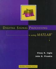
A thorough, hands-on treatment of DSP concepts implemented directly in MATLAB, making it the standard reference for anyone working in signals, communications, or audio engineering.

Covers control systems theory with strong MATLAB integration, connecting the mathematical framework to simulation and design — ideal for engineers working in dynamics and automation.
Advanced Mastery: Scientific Computing and Simulation
ExpertTackle advanced topics including partial differential equations, optimization, large-scale simulation, and the boundary between MATLAB and production-level scientific computing.
▸ Study plan for this stage
Pace: 8–10 weeks, ~40–50 pages/day, with 2–3 days per week dedicated to hands-on implementation and debugging
- Finite Difference and Finite Element Methods (FDM/FEM) for discretizing PDEs
- Numerical stability, convergence analysis, and error estimation in PDE solvers
- MATLAB's vectorization and sparse matrix operations for large-scale scientific computing
- Optimization algorithms (gradient descent, Newton's method, constrained optimization) and their implementation
- Time-stepping schemes (explicit/implicit Euler, Runge-Kutta) for transient PDE problems
- Boundary conditions, domain decomposition, and handling complex geometries in simulations
- Performance profiling, memory management, and scalability limits of MATLAB for production code
- Interfacing MATLAB with compiled languages (C/Fortran) for computationally intensive kernels
- How do you discretize a 2D heat equation using finite differences, and what stability constraints (CFL conditions) must you satisfy?
- What are the trade-offs between explicit and implicit time-stepping schemes, and when should you use each in MATLAB?
- How do you formulate and solve a constrained optimization problem in MATLAB, and what role does the Hessian play in convergence?
- Explain how sparse matrix storage and vectorized operations reduce both memory and computation time in large-scale PDE solvers.
- What are the main performance bottlenecks when scaling a MATLAB PDE solver, and when should you consider rewriting critical sections in C or Fortran?
- How do boundary conditions affect the structure of your discretized system, and how do you enforce them in a finite difference or finite element code?
- Implement a 1D heat equation solver using explicit Euler time-stepping and finite differences; verify convergence by halving grid spacing and time step.
- Solve a 2D Poisson equation with Dirichlet boundary conditions using sparse matrices; compare direct (backslash) and iterative (GMRES, CG) solvers for speed and memory.
- Build a nonlinear PDE solver (e.g., Fisher's equation or a reaction-diffusion system) using implicit time-stepping and Newton's method for each time step.
- Implement a constrained optimization problem (e.g., minimize a quadratic form subject to linear or box constraints) using MATLAB's Optimization Toolbox; document the algorithm and convergence history.
- Profile and optimize a PDE solver using MATLAB's Profiler; identify bottlenecks, convert hot loops to vectorized operations, and measure speedup.
- Write a MEX function (C/Fortran interface) to accelerate a computationally expensive kernel (e.g., matrix-vector product or stencil computation) and benchmark against pure MATLAB.
Next up: This stage equips you with the mathematical and computational foundations to recognize when MATLAB reaches its limits and to make informed decisions about transitioning to production-level scientific computing frameworks, compiled languages, or specialized libraries—preparing you for the final stage of mastery.

While Python-focused, this book's rigorous treatment of PDE discretization and simulation concepts directly transfers to MATLAB workflows and is essential reading for serious scientific computing.

Consolidates advanced numerical techniques — optimization, sparse matrices, FFT, and symbolic computation — into a single MATLAB-centric reference that ties together everything from earlier stages.
Discussion
Keep reading
Paths that share books, cover the same subject, or open a related topic.