Learn numerical methods: the best books in order
This curriculum builds a rigorous, practical mastery of numerical methods starting from a solid intermediate foundation — assuming comfort with calculus and linear algebra — and progressing through core algorithms, analysis, and finally advanced topics like differential equations and iterative solvers. Each stage sharpens both the mathematical theory and the computational intuition needed to implement and trust numerical algorithms.
Core Foundations
IntermediateEstablish a firm grasp of the essential numerical methods — root-finding, interpolation, numerical integration, and basic linear systems — along with error analysis and floating-point arithmetic.
▸ Study plan for this stage
Pace: 8–10 weeks, ~40–50 pages/day, with 2–3 days per week dedicated to problem-solving and coding exercises
- Floating-point representation, machine epsilon, and sources of numerical error (rounding, truncation, propagation)
- Root-finding methods: bisection, Newton-Raphson, secant method, and convergence criteria
- Polynomial interpolation: Lagrange and Newton forms, divided differences, and error bounds
- Numerical differentiation and integration: forward/backward/central differences, trapezoidal rule, Simpson's rule, and Gaussian quadrature
- Direct and iterative methods for solving linear systems: Gaussian elimination, LU decomposition, Jacobi, Gauss-Seidel, and convergence analysis
- Condition number and stability: understanding ill-conditioned systems and their practical implications
- Error analysis framework: absolute vs. relative error, order of accuracy, and Richardson extrapolation
- What is machine epsilon, and how does it limit the precision of floating-point arithmetic in practice?
- Compare the convergence rates and computational costs of bisection, Newton-Raphson, and secant methods for root-finding. When would you choose each?
- Explain the difference between Lagrange and Newton interpolation forms, and why divided differences are useful for constructing interpolating polynomials.
- Derive or explain the error bounds for polynomial interpolation and numerical integration, and how they depend on the function's derivatives.
- What is the condition number of a matrix, and why is it critical for assessing the reliability of solutions to linear systems?
- Describe the trade-offs between direct methods (Gaussian elimination) and iterative methods (Jacobi, Gauss-Seidel) for solving large linear systems.
- Implement bisection, Newton-Raphson, and secant methods in Python/MATLAB; solve 5–10 test problems and compare convergence rates empirically.
- Write code to compute Lagrange and Newton interpolating polynomials; test on a known function and verify error bounds match theory.
- Implement numerical differentiation (forward, backward, central differences) and study how step size affects accuracy; demonstrate the optimal step size phenomenon.
- Code the trapezoidal rule, Simpson's rule, and Gaussian quadrature; integrate 5 test functions and compare accuracy vs. computational cost.
- Implement Gaussian elimination with partial pivoting and LU decomposition; solve a system of 10–20 equations and verify the solution.
- Implement Jacobi and Gauss-Seidel iterative solvers; test convergence on both well-conditioned and ill-conditioned systems; compute condition numbers.
- Analyze floating-point error propagation: compute a sum in forward and reverse order, and explain the difference using machine epsilon.
- Use Richardson extrapolation to improve the accuracy of a numerical derivative or integral estimate; compare with higher-order methods.
Next up: Mastery of these core methods and error analysis provides the foundation for advanced topics such as eigenvalue problems, nonlinear systems of equations, ordinary differential equations, and optimization—where the same principles of convergence, stability, and error control apply at greater complexity.

An ideal entry point at the intermediate level: it builds intuition for why numerical methods are needed, covers root-finding, interpolation, and integration with clear worked examples, and keeps theory grounded in practical application.

The canonical undergraduate-to-graduate bridge text. Read after Chapra to formalize the theory — convergence proofs, error bounds, and algorithmic rigor — across the same core topics, preparing you for deeper study.
Linear Algebra & Systems
IntermediateMaster the numerical treatment of linear and nonlinear systems — direct and iterative solvers, matrix factorizations, eigenvalue problems, and conditioning — which underpin nearly all advanced numerical work.
▸ Study plan for this stage
Pace: 8–10 weeks, ~40–50 pages/day (Trefethen: ~3 weeks; Golub: ~5–7 weeks)
- Vector and matrix norms, condition numbers, and their role in measuring numerical stability and error propagation
- LU, QR, and Cholesky factorizations—their computational costs, numerical properties, and when to use each
- Direct solvers for linear systems: Gaussian elimination, pivoting strategies, and backward stability analysis
- Iterative solvers (GMRES, CG, BiCG) and convergence theory—when to prefer them over direct methods
- Eigenvalue problems: power iteration, QR algorithm, and Krylov subspace methods (Arnoldi, Lanczos)
- Matrix perturbation theory and backward error analysis—understanding how small input changes affect solutions
- Sparse matrix techniques and computational complexity—exploiting structure for efficiency
- Nonlinear systems and Newton's method—extending linear algebra insights to nonlinear problems
- What is the condition number of a matrix, how is it computed, and why does it determine the sensitivity of linear system solutions to perturbations?
- Compare LU, QR, and Cholesky factorizations: what are their computational costs, stability properties, and appropriate use cases?
- Explain the difference between direct and iterative solvers for linear systems, and describe when you would choose each approach.
- How does the QR algorithm compute eigenvalues, and what is the role of Hessenberg reduction in making it efficient?
- What is backward stability, and why is it more important than forward error analysis in numerical linear algebra?
- Describe the Arnoldi and Lanczos processes: how do they build Krylov subspaces, and why are they useful for eigenvalue and linear system problems?
- Implement Gaussian elimination with partial pivoting from scratch; compare numerical stability against a library solver (e.g., NumPy) on ill-conditioned systems
- Compute LU, QR, and Cholesky factorizations by hand for small matrices (3×3 or 4×4); verify backward stability by computing residuals
- Write code to compute condition numbers using different norms; test how condition number predicts error growth in solving Ax=b with perturbed A and b
- Implement the power iteration method and the QR algorithm for eigenvalue problems; apply to a 5×5 matrix and compare results to library eigensolvers
- Code a basic GMRES or CG solver for a sparse linear system; compare convergence rates and computational cost against a direct solver
- Analyze a real sparse matrix (e.g., from a finite difference discretization); implement reordering strategies (e.g., reverse Cuthill–McKee) and measure impact on factorization fill-in
- Solve a nonlinear system using Newton's method; compute the Jacobian numerically and analytically; study convergence behavior near and far from solutions
- Perform backward error analysis on a computed solution to Ax=b: compute ||Ax−b|| and ||A||·||x||·ε_machine; verify the backward error is small even when forward error is large
Next up: This stage equips you with the foundational linear algebra machinery and stability analysis tools needed to tackle approximation theory, optimization, and differential equations—where you'll apply these solvers and conditioning insights to continuous problems.

A beautifully concise and modern treatment of matrix algorithms, SVD, QR, and iterative methods. Its lecture-style format builds deep geometric and algebraic intuition that purely algorithmic books miss.
The definitive reference for numerical linear algebra algorithms. Read after Trefethen to go deeper into implementation details, stability analysis, and the full breadth of factorization and eigenvalue methods.
Approximation, Interpolation & Integration
IntermediateDevelop a thorough understanding of polynomial and spline approximation, quadrature theory, and spectral methods — the mathematical machinery behind accurate function representation and integration.
▸ Study plan for this stage
Pace: 8–10 weeks, ~40–50 pages/day (Hamming: 4–5 weeks; Trefethen: 4–5 weeks)
- Polynomial interpolation (Lagrange, Newton, Chebyshev bases) and the role of node placement in accuracy
- Error analysis in approximation: convergence rates, Runge phenomenon, and conditioning
- Spline approximation (cubic splines, B-splines) as a practical alternative to high-degree polynomials
- Quadrature theory: Newton–Cotes formulas, Gaussian quadrature, and adaptive integration
- Orthogonal polynomials (Legendre, Chebyshev, Hermite) and their connection to optimal approximation
- Spectral methods: using orthogonal expansions (Fourier, Chebyshev) for function representation and solving differential equations
- Practical trade-offs: balancing accuracy, computational cost, and numerical stability in real applications
- Function approximation as a foundational tool for solving PDEs and engineering problems
- Why does Chebyshev interpolation avoid the Runge phenomenon, and how does node placement affect polynomial interpolation accuracy?
- What is the difference between polynomial interpolation and spline approximation, and when should you use each?
- How do Gaussian quadrature rules achieve higher accuracy than Newton–Cotes formulas, and what role do orthogonal polynomials play?
- Explain the connection between orthogonal polynomials, least-squares approximation, and spectral methods.
- How do you construct and analyze cubic splines, and what makes them numerically stable?
- What are the convergence rates for polynomial, spline, and spectral approximations, and how do they compare?
- Implement Lagrange and Newton polynomial interpolation; compare accuracy and computational cost on test functions (e.g., Runge's function, smooth functions).
- Construct Chebyshev nodes for polynomial interpolation and verify that they eliminate the Runge phenomenon compared to equally-spaced nodes.
- Build a cubic spline interpolant from scratch (natural, clamped, and periodic boundary conditions); test on non-smooth data and compare to polynomial interpolation.
- Implement Newton–Cotes quadrature rules (trapezoidal, Simpson's) and Gaussian quadrature; measure convergence rates on integrals of varying smoothness.
- Write code to compute orthogonal polynomial expansions (Legendre, Chebyshev) and use them to approximate functions; analyze truncation error vs. degree.
- Solve a 1D boundary-value problem using spectral collocation with Chebyshev polynomials; compare accuracy and speed to finite-difference methods.
- Implement adaptive quadrature (e.g., adaptive Simpson's rule) and test on functions with localized features; measure efficiency gains.
- Perform error analysis: compute condition numbers for polynomial interpolation matrices at different node distributions and relate to observed numerical errors.
Next up: Mastery of approximation, interpolation, and integration techniques provides the mathematical foundation for solving differential equations numerically—the next stage will apply these tools to initial-value problems, boundary-value problems, and PDEs.
A classic that goes beyond recipes to explain *why* algorithms work, with deep insight into approximation and the philosophy of numerical computation — essential reading before tackling spectral and advanced quadrature methods.

A modern, rigorous treatment of polynomial approximation and Chebyshev methods, directly connected to practical computation via Chebfun. It bridges classical theory and state-of-the-art numerical practice.
Differential Equations — ODEs & PDEs
ExpertGain mastery over the numerical solution of ordinary and partial differential equations, including stability analysis, stiff systems, finite difference and finite element methods.
▸ Study plan for this stage
Pace: 12–14 weeks, ~40–50 pages/day (with 2–3 days/week dedicated to implementation and exercises)
- Initial value problems (IVPs) and boundary value problems (BVPs) for ODEs; Runge-Kutta methods, multistep methods, and their convergence/stability properties
- Stiff differential equations: recognition, implicit methods (backward Euler, BDF), and adaptive step-size control for efficient integration
- Finite difference methods for PDEs: discretization of elliptic, parabolic, and hyperbolic equations; consistency, stability (CFL condition, von Neumann analysis), and convergence
- Finite element method (FEM) fundamentals: weak formulations, basis functions, assembly of global systems, and error estimation
- Stability analysis: absolute stability regions, A-stability, L-stability; eigenvalue analysis for spatial discretizations
- Practical implementation: handling boundary conditions, nonlinear systems arising from discretization, and choosing appropriate solvers
- Finite element applications to PDEs: Galerkin methods, variational formulations, and extension to nonlinear and time-dependent problems
- Computational efficiency: sparse matrix techniques, iterative solvers, and trade-offs between accuracy and computational cost
- What are the key differences between explicit and implicit ODE methods, and when should each be used? How do stability regions guide this choice for stiff systems?
- Explain the CFL condition and von Neumann stability analysis for finite difference discretizations of PDEs. Why is stability analysis essential before implementation?
- How does the finite element method differ from finite differences? What is the role of weak formulations and basis functions in FEM?
- Describe the process of assembling a global finite element system from element-level contributions. How are boundary conditions incorporated?
- What makes a differential equation 'stiff,' and why do standard explicit methods fail? How do methods like BDF address this challenge?
- Given a PDE (e.g., heat equation or wave equation), outline the steps to discretize it using finite differences or finite elements, analyze stability, and implement a solver.
- Implement Runge-Kutta methods (RK2, RK4) and a multistep method (e.g., Adams-Bashforth) for a non-stiff IVP; compare accuracy and step-size requirements.
- Solve a stiff ODE system (e.g., Robertson's problem or a chemical kinetics model) using both explicit (RK4) and implicit (backward Euler or BDF) methods; measure CPU time and accuracy to demonstrate the stiffness problem.
- Discretize the 1D heat equation using finite differences (forward/backward Euler in time, central differences in space); implement von Neumann stability analysis and verify CFL constraints experimentally.
- Solve a 2D elliptic PDE (e.g., Poisson equation) on a rectangular domain using finite differences; implement a sparse direct or iterative solver and visualize the solution.
- Implement a basic finite element solver for a 1D boundary value problem (e.g., −u″ + u = f with Dirichlet BCs); use piecewise linear elements and assemble the global stiffness matrix.
- Extend the 1D FEM solver to a 2D problem (e.g., Poisson equation on a triangular mesh); use a mesh generation tool or simple structured mesh and compare FEM results to finite difference solutions.
Next up: This stage equips you with the foundational numerical techniques and stability theory needed to tackle advanced topics such as adaptive methods, multigrid solvers, spectral methods, and applications to complex real-world PDEs in the next stage.

A focused, mathematically careful treatment of ODE solvers — Runge-Kutta, multistep methods, stiffness, and stability — that builds directly on the analysis tools developed in earlier stages.
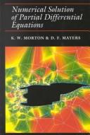
A rigorous and comprehensive introduction to finite difference methods for PDEs, covering stability (von Neumann analysis), consistency, and convergence — the natural next step after mastering ODEs.
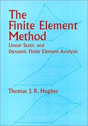
The authoritative text on finite element methods for PDEs. Read last in this stage to see how variational formulations and FEM extend and complement the finite difference approach for complex geometries.
Advanced Analysis & Modern Perspectives
ExpertSynthesize everything into a unified, rigorous mathematical framework — understanding convergence, stability, and complexity at a research-ready level, and connecting classical methods to modern scientific computing.
▸ Study plan for this stage
Pace: 12–16 weeks, ~40–50 pages/day (Quarteroni: 6–8 weeks, ~45 pages/day; Higham: 5–7 weeks, ~40 pages/day)
- Unified framework of convergence analysis: consistency, stability, and Lax equivalence theorem across all major method classes (ODEs, PDEs, linear systems)
- Rounding error propagation and backward error analysis: how machine arithmetic affects algorithm reliability and when methods remain stable despite perturbations
- Condition numbers and sensitivity: quantifying problem ill-conditioning and designing algorithms robust to data uncertainty
- Stability regions and absolute stability for time-stepping: understanding when explicit/implicit methods succeed or fail for stiff and oscillatory problems
- Complexity-accuracy trade-offs: balancing computational cost, convergence rates, and error tolerances in modern scientific computing
- Structured perturbation theory: analyzing how errors in matrix factorizations, eigenvalue computations, and linear solvers propagate through applications
- Modern perspectives on classical methods: connecting finite differences, finite elements, and spectral methods through variational and functional-analytic foundations
- Practical algorithm design: choosing methods based on rigorous stability and accuracy guarantees rather than heuristics
- Explain the Lax equivalence theorem and how it unifies convergence analysis for consistent, stable discretizations of PDEs and time-dependent problems.
- What is backward error analysis, and why is it more informative than forward error analysis for assessing algorithm reliability in floating-point arithmetic?
- Define the condition number of a problem and a matrix. How do they relate, and what do they tell you about algorithm design choices?
- Describe the absolute stability region of a numerical method for ODEs. Why do implicit methods have larger stability regions than explicit methods, and when does this matter?
- How do rounding errors accumulate in Gaussian elimination, and what does the growth factor tell you about pivot selection strategies?
- Compare the convergence properties of finite difference, finite element, and spectral methods for a PDE problem you choose. What are the trade-offs?
- Given a stiff ODE system, explain how you would choose between explicit and implicit methods, and what role stability regions play in that decision.
- What is structured perturbation analysis, and how does it improve upon classical error bounds for matrix computations?
- Implement Gaussian elimination with partial pivoting and measure the growth factor for random and pathological matrices; verify that the growth factor bounds the backward error.
- Solve a stiff ODE (e.g., Robertson problem) using explicit (RK4) and implicit (BDF) methods; plot stability regions and verify that implicit methods handle large time steps where explicit methods fail.
- Compute condition numbers for ill-conditioned linear systems (e.g., Hilbert matrices) and solve them using direct and iterative methods; compare forward and backward errors.
- Discretize a 1D or 2D PDE (e.g., heat equation, Poisson) using finite differences, finite elements, and (if feasible) spectral methods; analyze convergence rates empirically and compare to theory.
- Perform a backward error analysis for a simple algorithm (e.g., dot product, matrix-vector multiplication) in floating-point arithmetic; compute the condition number and verify error bounds.
- Implement a Krylov subspace method (GMRES or CG) for a large sparse system; study how preconditioning affects convergence and relate it to the spectrum of the preconditioned matrix.
- Analyze the stability of a multistep method (e.g., BDF or Adams) by plotting its stability region; apply it to a test problem and verify the predicted behavior.
- Study a research paper on modern scientific computing (e.g., on structure-preserving algorithms or high-order methods) and write a 2–3 page summary connecting its results to Quarteroni and Higham's frameworks.
Next up: This stage equips you with the rigorous mathematical and computational foundations to critically evaluate, design, and analyze specialized numerical methods for your own research or advanced applications—whether in machine learning, climate modeling, quantum computing, or other domains requiring provably reliable algorithms.

A graduate-level synthesis that unifies all major areas — linear systems, eigenvalues, approximation, ODEs, and PDEs — with full mathematical rigor, making it the ideal capstone for the entire curriculum.

The deepest treatment of floating-point arithmetic, rounding error analysis, and algorithm stability available. Read last to critically evaluate every algorithm encountered throughout the curriculum.
Discussion
Keep reading
Paths that share books, cover the same subject, or open a related topic.