The Best Operations Research Books, in Order
This curriculum is designed for expert-level learners who already possess strong mathematical maturity and want to achieve deep, research-grade mastery of operations research. The path moves from rigorous theoretical foundations in linear programming and optimization, through the analytical machinery of stochastic processes and queuing, and culminates in advanced decision modeling and integer/nonlinear programming — each stage building directly on the tools and vocabulary of the last.
Rigorous Foundations: Linear Programming & Duality
ExpertAchieve a deep, proof-level understanding of linear programming, the simplex method, duality theory, and sensitivity analysis — the bedrock of all classical OR.
▸ Study plan for this stage
Pace: 8–10 weeks, ~40–50 pages/day (mix of theory and worked solutions)
- Polyhedra, vertices, and basic feasible solutions as geometric foundations of LP
- The simplex method: pivoting rules, degeneracy, cycling prevention, and computational complexity
- Strong duality theorem and complementary slackness conditions
- Sensitivity analysis: shadow prices, ranges of optimality, and parametric programming
- Conic duality and the role of dual feasibility in proving optimality
- Revised simplex method and computational efficiency
- Degeneracy resolution strategies (Bland's rule, perturbation methods)
- Integer programming relaxations and LP's role in branch-and-bound
- Why are vertices of the feasible region optimal solutions, and how does the simplex method exploit this geometric insight?
- Prove the strong duality theorem: under what conditions is the optimal value of the primal equal to the optimal value of the dual?
- What is complementary slackness, and how do you use it to verify optimality or construct dual solutions from primal ones?
- How does sensitivity analysis quantify the value of relaxing a constraint, and what are the limits of the shadow price interpretation?
- Explain the revised simplex method and why it is computationally superior to the standard simplex for large sparse problems.
- What causes cycling in the simplex method, and how do Bland's rule and perturbation methods prevent it?
- Given a primal LP and its dual, construct the dual problem and verify that weak duality holds.
- Work through 15–20 complete simplex tableaus from Chvátal's solutions manual, tracking basis changes and identifying degenerate pivots.
- Construct the dual of at least 5 different primal LPs (standard form, inequality form, mixed constraints) and verify weak duality by hand.
- Solve a parametric LP where the RHS or objective coefficients vary, determine the breakpoints, and sketch the optimal value function.
- Implement or trace through the revised simplex method on a 5×8 problem; compare computational steps to the standard method.
- Prove complementary slackness for a specific primal–dual pair and use it to verify optimality without re-solving.
- Identify a degenerate LP, apply Bland's rule to prevent cycling, and compare with an arbitrary pivot rule.
- Perform a complete sensitivity analysis on a 3–4 variable LP: compute shadow prices, ranges of optimality for objective coefficients, and ranges for RHS values.
- Formulate and solve a small integer program by relaxing it to LP, interpreting the dual, and using LP bounds in a branch-and-bound sketch.
Next up: This stage equips you with the theoretical and computational mastery of LP and duality needed to understand how these tools extend to network flows, integer programming, convex optimization, and stochastic OR—the advanced applications that follow.
The gold standard rigorous treatment of LP for experts. Chvátal develops the simplex method, duality, and degeneracy with full mathematical precision, building the exact vocabulary needed for everything that follows.

Complements Chvátal with a modern, unified view of LP, duality, and the geometry of polyhedra, and bridges cleanly into network flows and integer programming covered in later stages.
Network Flows, Integer Programming & Combinatorial Optimization
ExpertMaster the theory and algorithms for network flow problems, integer programming formulations, branch-and-bound, and cutting-plane methods — the core of discrete OR.
▸ Study plan for this stage
Pace: 8–10 weeks, ~40–50 pages/day (alternating between Ahuja's Network Flows and Wolsey's Integer Programming; expect 2–3 weeks per major topic cluster)
- Maximum flow and minimum cut: Ford-Fulkerson, push-relabel, and scaling algorithms; the max-flow min-cut theorem and its applications
- Minimum-cost flow: successive shortest paths, cycle canceling, and network simplex; modeling diverse logistics and routing problems as MCF
- Integer programming formulations: converting combinatorial problems into IP models; recognizing problem structure (assignment, knapsack, set cover, TSP)
- Linear programming relaxations and bounds: LP relaxation as a tool for bounding IP optimal values; understanding the integrality gap
- Branch-and-bound framework: tree search, node selection, variable selection, and pruning strategies; computational complexity and practical heuristics
- Cutting-plane methods: Gomory cuts, valid inequalities, and separation problems; strengthening LP relaxations to tighten bounds
- Polyhedral combinatorics: facets, valid inequalities, and the convex hull of feasible integer solutions; understanding problem structure through polytopes
- Practical modeling and algorithm selection: when to use network flow vs. IP; recognizing special structure (totally unimodular matrices, network matrices) for efficient solution
- Explain the max-flow min-cut theorem and derive a minimum cut from a maximum flow solution. How does this relate to the feasibility of a flow network?
- Compare and contrast the Ford-Fulkerson method, push-relabel algorithm, and scaling algorithms for maximum flow. What are the time complexities and when is each preferred?
- Formulate a traveling salesman problem, assignment problem, and set cover problem as integer programs. Identify the constraints and objective, and discuss their LP relaxations.
- Describe the branch-and-bound algorithm: how are bounds computed, nodes selected, and variables chosen for branching? What pruning strategies reduce the search tree?
- What is a cutting-plane method and how does it strengthen an LP relaxation? Give an example of a valid inequality (e.g., Gomory cut) and explain its geometric interpretation.
- When is a matrix totally unimodular (TU)? Why does an IP with a TU constraint matrix have an integral optimal LP solution? Give two examples of TU matrices.
- Solve a small minimum-cost flow problem by hand using successive shortest paths or cycle canceling. Verify optimality using complementary slackness.
- Design a branch-and-bound tree for a small integer program (e.g., 0–1 knapsack or facility location). Show LP relaxations, bounds, and pruning decisions at each node.
- Implement the Ford-Fulkerson algorithm (with DFS or BFS augmentation) on a 5–8 node flow network; compute maximum flow and identify a minimum cut. Verify the max-flow min-cut theorem.
- Implement a push-relabel or scaling algorithm for maximum flow; compare runtime and node/edge operations against Ford-Fulkerson on a medium-sized instance (20–50 nodes).
- Formulate and solve (by hand or with a solver) a minimum-cost flow problem from a real application (e.g., transportation, supply-demand matching). Use successive shortest paths or the network simplex method.
- Formulate a combinatorial optimization problem (TSP, assignment, set cover, facility location) as an integer program; solve its LP relaxation and compare the bound to known optimal values.
- Implement a basic branch-and-bound algorithm for a 0–1 knapsack or small integer program; track the search tree, LP bounds, and pruning. Document which nodes are pruned and why.
- Generate Gomory cuts for a small integer program (2–3 variables, 2–3 constraints); add cuts to the LP relaxation and observe the tightening of the bound.
- Analyze the constraint matrix of a network flow problem and verify total unimodularity (TU) using the characterization from Wolsey; explain why the LP optimal is integral.
- Solve a small TSP instance (8–10 cities) using branch-and-bound with LP relaxations (Held-Karp lower bound or assignment LP); document the search tree and final solution.
Next up: This stage equips you with the algorithmic and theoretical foundations of discrete optimization—network flows, integer programming, and polyhedral methods—which are essential prerequisites for advanced topics such as approximation algorithms, heuristics, metaheuristics, and specialized algorithms for specific problem classes (scheduling, routing, facility location).
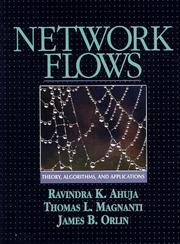
The definitive reference on network optimization; covers shortest paths, max-flow, min-cost flow, and matching with full algorithmic rigor, providing essential structure for integer programming.
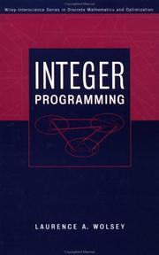
The canonical expert-level text on IP: formulations, relaxations, cutting planes, and branch-and-bound are treated with the depth and precision needed for serious research or practice.
Nonlinear & Convex Optimization
ExpertDevelop mastery of convex analysis, KKT conditions, duality in nonlinear settings, and modern first- and second-order algorithms for continuous optimization.
▸ Study plan for this stage
Pace: 12–14 weeks, ~40–50 pages/day (Boyd first 6–7 weeks, Bertsekas 5–7 weeks)
- Convex sets, convex functions, and convex optimization problems (Boyd Ch. 2–3)
- Lagrange duality, KKT conditions, and optimality characterization (Boyd Ch. 5; Bertsekas Ch. 3–4)
- Subgradients, subdifferentials, and non-smooth convex analysis (Boyd Ch. 5; Bertsekas Ch. 5)
- Gradient descent, accelerated methods, and proximal algorithms (Boyd Ch. 9; Bertsekas Ch. 2)
- Newton's method, quasi-Newton methods, and second-order algorithms (Boyd Ch. 9–10; Bertsekas Ch. 1–2)
- Constraint qualification, regularity conditions, and duality gaps (Bertsekas Ch. 3–4)
- Interior-point methods and barrier methods (Boyd Ch. 11)
- Stochastic gradient methods and online optimization (Bertsekas Ch. 6)
- What is a convex set and a convex function, and why does convexity guarantee that any local minimum is global?
- State the KKT conditions and explain when they are necessary and sufficient for optimality in constrained nonlinear programs.
- What is Lagrange duality, and how does strong duality relate to constraint qualification and the duality gap?
- Derive and explain the subgradient of a non-smooth convex function; when does it reduce to the gradient?
- Compare gradient descent, accelerated gradient methods (e.g., Nesterov), and Newton's method in terms of convergence rate and computational cost.
- How do interior-point methods work, and what is the role of the barrier parameter in solving constrained problems?
- Explain the difference between batch gradient descent and stochastic gradient descent, and when each is appropriate.
- Work through Boyd Ch. 2–3 exercises: verify convexity of given functions using definitions, epigraph characterization, and composition rules.
- Solve 5–8 constrained optimization problems by hand: formulate the Lagrangian, compute KKT conditions, and verify optimality.
- Implement gradient descent and accelerated gradient descent (Nesterov) in Python on 3–4 test functions (e.g., quadratic, Rosenbrock); compare convergence curves.
- Code Newton's method and a quasi-Newton method (BFGS) for unconstrained problems; benchmark against gradient-based methods on medium-scale problems.
- Implement a proximal gradient algorithm for a composite problem (e.g., ℓ1-regularized least squares); verify convergence and compare to standard methods.
- Solve 3–4 problems from Bertsekas Ch. 3–4 on duality and constraint qualification; construct examples where strong duality fails.
- Implement an interior-point method (or use a library like CVXPY) to solve a constrained QP and a nonlinear program; analyze the barrier parameter's effect.
- Apply stochastic gradient descent to a large-scale problem (e.g., logistic regression on a real dataset); tune step size and batch size; compare to batch methods.
Next up: This stage equips you with the theoretical foundations and algorithmic toolkit for continuous optimization, enabling you to tackle distributed optimization, online learning, and large-scale machine learning problems in the next stage.

The essential modern reference for convex optimization; its unified treatment of duality, optimality conditions, and problem classes (SOCPs, SDPs) is indispensable for advanced OR work.
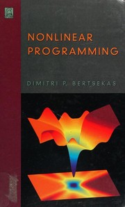
Provides the rigorous theoretical backbone — Lagrangian duality, penalty methods, gradient and Newton methods — that Boyd's applied focus leaves implicit, cementing expert-level understanding.
Stochastic Processes & Queueing Theory
ExpertDeeply understand Markov chains, Poisson processes, and the analytical theory of queues (M/M/1 through G/G/1), enabling rigorous modeling of stochastic OR systems.
▸ Study plan for this stage
Pace: 8–10 weeks, ~40–50 pages/day (Wolff first 3 weeks, then Gross for remaining 5–7 weeks, with overlap for integration)
- Markov chains: state space, transition probabilities, classification of states (transient, recurrent, absorbing), and long-run behavior via Chapman-Kolmogorov equations
- Poisson processes: definition via counting processes, memoryless property, inter-arrival and service time distributions, and superposition/thinning
- Continuous-time Markov chains (CTMCs): generator matrices, balance equations, and steady-state solutions
- M/M/1 queue: arrival and service processes, traffic intensity, queue length and waiting time distributions, Little's Law
- M/M/c and M/M/∞ systems: multi-server queues, Erlang C formula, and capacity planning
- General arrival/service models (M/G/1, G/M/1, G/G/1): Pollaczek-Khintchine formula, bounds, and approximations
- Network of queues: Jackson networks, product-form solutions, and decomposition methods
- Transient analysis and numerical methods: solving differential equations, simulation validation, and computational approaches
- What is the Chapman-Kolmogorov equation, and how does it characterize the evolution of a Markov chain? How do you use it to compute n-step transition probabilities?
- Define a Poisson process rigorously. Why is the memoryless property central to queueing theory, and how does it simplify analysis of M/M/1 systems?
- Derive the steady-state distribution for an M/M/1 queue from balance equations. What is the traffic intensity ρ, and what condition must it satisfy for stability?
- State and apply Little's Law (L = λW). How does it relate queue length, waiting time, and arrival rate, and why is it model-independent?
- Compare M/M/1, M/M/c, and M/G/1 queues: what are the key distributional differences, and how do you compute mean queue length and waiting time for each?
- What is the Pollaczek-Khintchine formula, and how does it extend M/M/1 results to M/G/1 systems? When is it exact vs. approximate?
- How do you analyze a Jackson network? What is the product-form solution, and under what conditions does it apply?
- Describe the balance equation method for finding steady-state probabilities in a CTMC. How does it differ from solving the generator matrix directly?
- Work through Wolff's examples of Markov chain classification (transient vs. recurrent states) for 2–3 small chains; compute absorption probabilities and expected hitting times by hand
- Simulate a Poisson arrival process with rate λ = 5/hour; verify empirically that inter-arrival times are exponential and that the counting process has independent increments
- Derive the steady-state distribution π for an M/M/1 queue with λ = 3 and μ = 5 using balance equations; compute L, Lq, W, Wq, and verify Little's Law
- Solve a multi-server M/M/c problem (e.g., c = 3, λ = 10, μ = 4 per server) using Erlang C formula; interpret the probability of waiting and compare to M/M/1
- Apply the Pollaczek-Khintchine formula to an M/G/1 queue with Erlang-2 service times; compute mean queue length and compare to simulation
- Analyze a small Jackson network (3–4 nodes) by computing arrival rates at each node and steady-state probabilities using product-form; validate via simulation
- Implement a numerical solver (e.g., Gaussian elimination or iterative method) to find steady-state probabilities for a CTMC with 5–10 states; compare to analytical results
- Model a real-world queueing scenario (e.g., bank teller, call center, hospital ER) as M/M/c or M/G/1; estimate parameters from data, compute performance metrics, and recommend staffing levels
Next up: This stage equips you with the analytical and computational foundations of stochastic modeling, enabling the next stage to extend these tools to optimization (capacity planning, staffing), simulation validation, and advanced network models (e.g., non-Markovian networks, priority queues, and control policies).
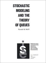
A rigorous, mathematically complete treatment of queueing theory grounded in renewal theory and Markov processes — the right starting point for expert-level stochastic OR.
Provides exhaustive coverage of queue models (bulk, priority, networks of queues) with analytical depth, serving as an essential reference alongside Wolff's theoretical framework.
Decision Modeling, Dynamic Programming & Stochastic Optimization
ExpertSynthesize all prior knowledge into advanced decision-making frameworks: dynamic programming, Markov decision processes, stochastic programming, and robust optimization.
▸ Study plan for this stage
Pace: 8–10 weeks, ~40–50 pages/day (Bertsekas Vol. I: ~600 pages over 5–6 weeks; Birge: ~400 pages over 3–4 weeks)
- Principle of optimality and the Bellman equation as the foundation for solving sequential decision problems
- Value iteration and policy iteration algorithms for computing optimal policies in finite and infinite-horizon problems
- Markov decision processes (MDPs): state spaces, transition probabilities, reward structures, and discount factors
- Stochastic dynamic programming: handling uncertainty through conditional expectations and scenario-based formulations
- Stochastic programming models (two-stage and multi-stage): recourse decisions, wait-and-see vs. here-and-now decisions
- Scenario trees and scenario generation for approximating continuous probability distributions
- Decomposition methods (Benders decomposition, Dantzig-Wolfe) for solving large-scale stochastic programs
- Robust optimization: uncertainty sets, minimax formulations, and trade-offs between optimality and feasibility under ambiguity
- How does the Bellman equation enable recursive decomposition of sequential decision problems, and what assumptions must hold for the principle of optimality to apply?
- What is the difference between value iteration and policy iteration, and when is each algorithm preferable in terms of convergence speed and computational cost?
- How do Markov decision processes formalize the structure of stochastic sequential decision problems, and what role do transition probabilities and discount factors play?
- In a two-stage stochastic program, what is the distinction between first-stage (here-and-now) and second-stage (wait-and-see) decisions, and how does the recourse function connect them?
- How do scenario trees approximate uncertainty in multi-stage stochastic programs, and what are the trade-offs between scenario granularity and computational tractability?
- What is the core idea behind Benders decomposition in stochastic programming, and how does it exploit the problem structure to enable parallel or iterative solution?
- How does robust optimization differ from stochastic programming in its treatment of uncertainty, and when is a minimax formulation more appropriate than a risk-based objective?
- Implement value iteration and policy iteration algorithms from scratch for a small finite-state MDP (e.g., inventory control or machine replacement) and compare convergence rates and final policy quality
- Formulate and solve a two-stage stochastic linear program (e.g., production planning with uncertain demand) using Birge's framework; generate 10–20 scenarios and solve with a commercial solver (CPLEX, Gurobi) or open-source tool (PuLP, Pyomo)
- Build a scenario tree for a multi-stage stochastic program (e.g., portfolio optimization over 3–5 periods) and implement a scenario-tree-based dynamic programming solution
- Solve a finite-horizon MDP using backward induction (Bertsekas Ch. 1–2 examples); verify the optimal policy by simulation under different initial states
- Implement Benders decomposition for a two-stage stochastic program: separate master (first-stage) and subproblems (second-stage), and iterate until convergence
- Formulate the same decision problem as both a stochastic program and a robust optimization problem; compare the optimal solutions and discuss the impact of uncertainty representation on decisions
Next up: This stage equips you with the mathematical and algorithmic foundations to model and solve real-world sequential decision problems under uncertainty; the next stage will apply these frameworks to specific domains (supply chain, finance, energy) and explore practical implementation, approximation methods, and scalability challenges.

The definitive two-volume treatment of DP and MDPs; its depth on exact and approximate methods, including reinforcement learning connections, makes it the capstone of deterministic and stochastic OR.
Covers two-stage and multi-stage stochastic programs, decomposition methods (L-shaped, Benders), and robust formulations — the frontier where optimization meets uncertainty, tying the entire curriculum together.
Discussion
Keep reading
Paths that share books, cover the same subject, or open a related topic.