The Best Books to Learn Mathematical Optimization, In Order
This curriculum is designed for expert-level learners who already have strong mathematical maturity and want to achieve deep mastery of mathematical optimization across its three major pillars: convex analysis, linear programming, and numerical methods. The path moves from rigorous theoretical foundations through algorithmic theory and into advanced computational and applied methodology, with each stage demanding and building upon the last.
Theoretical Foundations
ExpertBuild a rigorous, unified understanding of convex analysis and the mathematical structures that underpin all of optimization theory — duality, optimality conditions, and subdifferential calculus.
▸ Study plan for this stage
Pace: 8–10 weeks, ~40–50 pages/day (Chapters 1–11 of Boyd & Vandenberghe; ~600 pages core material)
- Convex sets and convex functions: definitions, properties, and geometric intuition behind why convexity enables global optimization
- Convex optimization problems: standard form, transformations, and the principle that any local minimum is global
- Duality theory: Lagrangian formulation, weak and strong duality, complementary slackness, and how dual problems provide bounds and insights
- Optimality conditions: KKT conditions as necessary and sufficient conditions for convexity, and their role in characterizing solutions
- Subdifferential calculus: subgradients, subdifferentials, and their use in non-smooth optimization and optimality characterization
- Conjugate functions and Fenchel duality: the dual perspective on functions and how it connects to duality theory
- Constraint qualifications and regularity conditions: when strong duality holds and when KKT conditions are sufficient
- Numerical algorithms as manifestations of theory: gradient descent, Newton's method, and interior-point methods grounded in convex analysis
- What is a convex set and a convex function, and why does convexity guarantee that any local minimum is a global minimum?
- State the KKT conditions for a convex optimization problem and explain when they are both necessary and sufficient for optimality.
- Define the Lagrangian dual problem and explain the relationship between weak duality, strong duality, and complementary slackness.
- What is a subgradient and a subdifferential, and how do they generalize the concept of a gradient to non-smooth functions?
- Explain the conjugate function and how Fenchel duality relates to the primal-dual structure of optimization problems.
- What constraint qualifications ensure that strong duality holds, and why are they necessary?
- Verify convexity of 5–10 functions from Boyd (e.g., norms, exponential, log-sum-exp) using definitions, Hessian tests, and composition rules; prove non-convexity of counterexamples.
- Formulate and solve 4–6 convex optimization problems in standard form (LP, QP, SOCP, SDP); transform non-standard problems into standard form using Boyd's techniques.
- Derive the Lagrangian dual for 5–8 problems of increasing complexity; compute weak and strong duality gaps; verify complementary slackness at optimal solutions.
- Compute KKT conditions for 6–8 problems; solve them analytically where possible; verify that solutions satisfy KKT and interpret the dual variables as shadow prices.
- Calculate subgradients and subdifferentials for 5–8 non-smooth functions (absolute value, max, indicator functions); verify optimality using subdifferential conditions.
- Compute conjugate functions for 4–6 examples; verify Fenchel duality relationships; use conjugates to reformulate and solve dual problems.
Next up: This stage establishes the mathematical bedrock—convex analysis, duality, and optimality conditions—that makes the next stage's focus on algorithms and applications both rigorous and intuitive, since you will now understand *why* algorithms work and *when* they are guaranteed to succeed.

Bridges pure convex analysis to optimization problems and algorithms with exceptional clarity; its treatment of duality and problem transformations is indispensable and provides the applied counterpart to Rockafellar.
Linear and Discrete Optimization
ExpertMaster the theory and algorithms of linear programming — simplex, duality, sensitivity analysis, and integer programming — at a level suitable for research and algorithm design.
▸ Study plan for this stage
Pace: 12–14 weeks, ~40–50 pages/day, with 2–3 days per week for problem-solving and algorithm implementation
- Simplex algorithm: pivoting rules, degeneracy, cycling prevention, and computational complexity
- Duality theory: weak and strong duality, complementary slackness, and dual interpretation of sensitivity
- Sensitivity analysis: shadow prices, ranging, and parametric programming
- Integer programming: cutting planes, branch-and-bound, and integrality gaps
- Polyhedra and polytopes: vertices, edges, faces, and the structure of feasible regions
- Totally unimodular matrices and their role in ensuring integer solutions
- Network flow problems and their connection to linear programming
- Computational complexity: polynomial-time solvability and hardness results for variants
- Explain the simplex algorithm step-by-step, including how pivoting works and why it terminates (or cycles under degeneracy)
- State and prove the weak and strong duality theorems; what does complementary slackness tell you about optimal solutions?
- Given a linear program, how would you compute shadow prices and use them to analyze the impact of constraint relaxation?
- What is the difference between linear and integer programming, and why is branch-and-bound necessary for integer programs?
- Describe the structure of polyhedra: what are vertices, edges, and faces, and how do they relate to basic feasible solutions?
- When does a linear program have an integer optimal solution without explicit integer constraints? What role do totally unimodular matrices play?
- Solve 5–10 small linear programs (3–5 variables, 3–4 constraints) by hand using the simplex algorithm; track all pivot operations and verify optimality conditions
- Formulate and solve the dual of 3–4 primal problems from the Solutions Manual; verify strong duality and complementary slackness conditions
- Implement the simplex algorithm in Python or Julia: code the tableau form, pivoting logic, and termination criteria; test on textbook examples
- Conduct sensitivity analysis on 2–3 solved LPs: compute ranges for objective coefficients and right-hand sides; interpret shadow prices economically
- Solve 4–6 integer programming problems using branch-and-bound by hand or with a simple implementation; compare LP relaxation bounds to integer optimum
- Analyze the constraint matrix of 2–3 problems for total unimodularity; verify whether the LP relaxation yields integer solutions
- Formulate a small network flow problem as an LP and solve it; verify that the optimal solution is integral without explicit integer constraints
Next up: This stage equips you with deep theoretical understanding and algorithmic mastery of linear and integer optimization, providing the foundation for advanced topics such as convex optimization, semidefinite programming, or specialized algorithms for combinatorial problems.
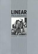
A rigorous yet accessible deep dive into the simplex method and LP theory; its proof-driven style builds the structural intuition needed before tackling more abstract formulations.

The definitive advanced reference unifying LP, integer programming, and polyhedral combinatorics; read after Chvátal to reach the research frontier of the field.
Nonlinear Optimization Theory
ExpertDevelop mastery of optimality conditions, constraint qualifications, and duality for general nonlinear programs, including both smooth and nonsmooth settings.
▸ Study plan for this stage
Pace: 8–10 weeks, ~40–50 pages/day (Bertsekas: weeks 1–5; Rockafellar: weeks 6–10)
- First-order and second-order optimality conditions (KKT conditions, Lagrange multipliers, constraint qualifications)
- Constraint qualifications (LICQ, MFCQ, CRCQ) and their role in ensuring KKT necessity and sufficiency
- Lagrangian duality and weak/strong duality for convex and nonconvex problems
- Subdifferential calculus and subgradients as generalizations of gradients in nonsmooth settings
- Variational inequalities and monotone operators as unifying frameworks for optimization
- Convex analysis foundations: convex sets, convex functions, and their properties
- Nonsmooth optimization theory and Clarke subdifferentials for nonsmooth functions
- Duality in variational analysis and its connection to optimization duality
- What are the KKT conditions, and under what constraint qualifications are they necessary and sufficient for optimality?
- How do LICQ, MFCQ, and CRCQ differ, and why does the choice of constraint qualification matter for optimization theory?
- Explain weak duality and strong duality: when does strong duality hold, and what does it tell us about primal and dual problems?
- What is a subdifferential, and how does it generalize the concept of a gradient to nonsmooth functions?
- How do variational inequalities unify optimization and fixed-point problems, and what role do monotone operators play?
- What is the relationship between convex conjugate functions and Lagrangian duality?
- Work through Bertsekas Chapter 3 (Convex Analysis) exercises: prove convexity of specific functions, compute subdifferentials of piecewise linear functions, and verify constraint qualifications on toy problems (e.g., quadratic programs with linear constraints).
- For a given nonlinear program (e.g., a constrained least-squares problem), compute the KKT conditions by hand, identify which constraint qualification holds, and verify whether KKT conditions are necessary/sufficient for optimality.
- Formulate the Lagrangian dual for a nonconvex problem from Bertsekas Chapter 5, compute the dual function, and compare primal and dual optimal values to understand the duality gap.
- Implement a simple subgradient method (from Bertsekas Chapter 2) on a nonsmooth convex function (e.g., ℓ₁ regularization) and observe convergence; compare with gradient descent on a smooth approximation.
- Study Rockafellar's treatment of Clarke subdifferentials (Chapter 2): compute Clarke subdifferentials for nonsmooth functions (e.g., max functions, absolute value compositions) and verify the calculus rules.
- Formulate a variational inequality for a given optimization problem (Rockafellar Chapter 12), identify the associated monotone operator, and solve it using a proximal or splitting method.
Next up: Mastery of optimality conditions, constraint qualifications, and duality in both smooth and nonsmooth settings provides the theoretical foundation for the next stage, which will focus on algorithmic methods (gradient descent, proximal algorithms, augmented Lagrangian methods) and their convergence analysis under these conditions.
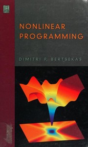
A mathematically thorough treatment of KKT theory, duality, and descent methods for nonlinear programs; Bertsekas's precise style makes this the gold standard for nonlinear theory at the expert level.
Extends classical convex analysis to nonsmooth and nonconvex settings via modern variational methods; essential for anyone pushing into research-level nonlinear or nonsmooth optimization.
Numerical Methods and Algorithms
ExpertAchieve deep understanding of the algorithmic machinery — interior-point methods, gradient methods, and large-scale solvers — including convergence analysis and implementation considerations.
▸ Study plan for this stage
Pace: 8–10 weeks, ~40–50 pages/day with 2–3 days per week for implementation and problem-solving
- Gradient descent and steepest descent methods: convergence rates, step-size selection, and practical implementation
- Newton's method and quasi-Newton methods (BFGS, L-BFGS): Hessian approximation, superlinear convergence, and memory-efficient variants
- Conjugate gradient methods: theory, preconditioning, and application to large sparse systems
- Interior-point methods: barrier functions, central path, duality, and polynomial-time complexity
- Line search and trust-region strategies: ensuring convergence, handling ill-conditioning, and practical algorithmic choices
- Constrained optimization: KKT conditions, penalty methods, and augmented Lagrangian approaches
- Large-scale solver design: matrix factorization, iterative methods, and computational complexity trade-offs
- Convergence analysis: linear, superlinear, and quadratic convergence; rates and practical stopping criteria
- What are the key differences between gradient descent, Newton's method, and quasi-Newton methods in terms of convergence rate and computational cost per iteration?
- How do interior-point methods maintain feasibility and ensure convergence along the central path, and why is this approach polynomial-time?
- Explain the role of line search and trust regions in ensuring global convergence, and when would you choose one over the other?
- What is the purpose of preconditioning in conjugate gradient methods, and how does it affect convergence?
- How do quasi-Newton methods (BFGS, L-BFGS) approximate the Hessian, and why is L-BFGS preferred for large-scale problems?
- Describe the KKT conditions and their role in characterizing optimal solutions for constrained problems.
- Implement steepest descent with backtracking line search on a quadratic function and a Rosenbrock function; compare convergence rates and iteration counts
- Code Newton's method for a small nonlinear system and verify superlinear convergence by plotting error vs. iteration
- Implement BFGS and L-BFGS on a 100+ dimensional problem; measure memory usage and wall-clock time compared to steepest descent
- Build a conjugate gradient solver from scratch for a sparse symmetric positive-definite system; test with and without diagonal preconditioning
- Implement a simple interior-point method for a small linear program or quadratic program; track the central path and verify barrier parameter reduction
- Solve a constrained optimization problem using both penalty methods and augmented Lagrangian; compare convergence behavior and solution quality
- Analyze convergence rates empirically: plot log(error) vs. iteration for different methods on the same test problem and identify linear vs. superlinear regimes
Next up: This stage equips you with rigorous understanding of the algorithmic foundations and convergence theory needed to evaluate, implement, and extend optimization solvers in practice—preparing you to tackle specialized applications, distributed algorithms, and advanced topics like stochastic optimization or nonconvex methods.
The definitive reference for numerical optimization algorithms — covering line search, trust region, conjugate gradient, quasi-Newton, and constrained methods — with rigorous convergence proofs and practical guidance.
Advanced Topics and Unification
ExpertSynthesize all prior knowledge into a unified, modern view of optimization — covering first-order methods at scale, operator splitting, and the deep connections between optimization, statistics, and computation.
▸ Study plan for this stage
Pace: 8–10 weeks, ~40–50 pages/day (mix of dense theory and worked examples; expect 2–3 hours daily for reading + reflection)
- First-order methods at scale: gradient descent, accelerated methods (Nesterov), proximal methods, and their convergence rates under different smoothness/strong convexity regimes
- Operator splitting and decomposition: ADMM, Douglas-Rachford, forward-backward splitting, and their role in distributed and large-scale optimization
- Duality and Lagrangian methods: understanding the dual problem structure, dual decomposition, and when duality gaps vanish (strong duality conditions)
- Stochastic optimization: SGD, variance reduction techniques (SVRG, SAG), and the interplay between sample complexity and iteration complexity
- Connections between optimization, statistics, and computation: how optimization algorithms relate to statistical estimation, convergence rates, and computational complexity theory
- Modern applications and scalability: handling non-smooth and composite objectives, distributed algorithms, and coordinate descent methods
- Subgradients and subdifferentials: extending calculus to non-smooth settings and their role in proximal and cutting-plane methods
- Complexity theory for optimization: lower bounds, oracle complexity, and the limits of first-order methods
- What are the convergence rates of gradient descent, accelerated gradient methods, and proximal methods under different assumptions (smoothness, strong convexity, Lipschitz continuity)? How do they compare?
- Explain operator splitting: what is the Douglas-Rachford algorithm, and how does ADMM generalize it? When is ADMM preferred over other decomposition methods?
- How do Lagrangian duality and dual decomposition enable distributed optimization? What conditions guarantee strong duality and zero duality gap?
- What is the role of variance reduction in stochastic optimization? How do SVRG and SAG improve upon vanilla SGD, and what are their iteration and sample complexities?
- How do optimization algorithms relate to statistical estimation? What is the connection between convergence rates of optimization algorithms and statistical rates of convergence?
- What are subgradients and subdifferentials, and why are they essential for handling non-smooth objectives? How do they appear in proximal methods and cutting-plane algorithms?
- What does oracle complexity tell us about the fundamental limits of first-order methods? Can you interpret lower bounds for convex optimization?
- Implement gradient descent, Nesterov accelerated gradient, and proximal gradient descent from scratch on a suite of test problems (quadratic, logistic regression, ℓ1-regularized least squares). Plot convergence curves and verify theoretical rates.
- Derive and implement the ADMM algorithm for a composite problem (e.g., ℓ1-regularized regression, matrix completion). Compare convergence speed and solution quality against proximal methods.
- Work through a dual decomposition example (e.g., distributed consensus or resource allocation) and implement both the primal and dual algorithms. Verify that the duality gap closes.
- Implement SGD with variance reduction (SVRG or SAG) on a large-scale dataset and compare iteration and sample complexity against vanilla SGD. Measure wall-clock time and final accuracy.
- Solve a non-smooth optimization problem using subgradient methods and proximal methods. Compute subgradients by hand for at least two objectives (e.g., ℓ1 norm, max function) and verify they satisfy the subdifferential definition.
- Implement coordinate descent or a distributed first-order method (e.g., federated averaging) on a realistic problem. Analyze how the method scales with problem dimension and number of agents.
- Prove or verify a convergence rate result from one of the books: choose a theorem, work through the proof, and implement the algorithm to confirm the predicted rate empirically.
- Write a short essay (2–3 pages) connecting an optimization algorithm to a statistical estimation problem: explain how the optimization convergence rate translates to statistical guarantees (e.g., sample complexity for learning).
Next up: This stage unifies optimization theory with modern computational practice and statistical foundations, positioning you to tackle specialized applications (e.g., machine learning, control, signal processing) and emerging areas (e.g., federated learning, online optimization, or optimization under uncertainty) where these principles are applied at scale.

Provides a unified, modern treatment of first-order and proximal algorithms, subgradient methods, and decomposition — the ideal capstone that ties together convex theory and numerical practice.
Covers conic optimization, robust optimization, and semidefinite programming — advanced modeling paradigms that extend beyond classical LP and NLP and represent the current frontier of applied optimization.
Discussion
Keep reading
Paths that share books, cover the same subject, or open a related topic.