The Best Books to Learn Mathematical Modeling, In Order
This curriculum builds genuine mastery of mathematical modeling by moving from structured problem-solving frameworks and classical techniques, through differential-equation and simulation-based modeling, to advanced stochastic and optimization-driven approaches. Because the learner starts at the intermediate level, early stages sharpen core modeling intuition before later stages demand rigorous analysis and computational depth.
Modeling Mindset & Core Frameworks
IntermediateDevelop a disciplined modeling process — how to translate a messy real-world problem into clean mathematical structure — and build fluency with the most common modeling archetypes.
▸ Study plan for this stage
Pace: 8–10 weeks, ~25–30 pages/day (alternating between conceptual reading and hands-on modeling work)
- The modeling cycle: problem formulation, model construction, model analysis, and interpretation/validation
- Dimensional analysis and scaling as tools to constrain and simplify models before detailed mathematics
- Linear and nonlinear differential equation models (population growth, decay, mixing, motion)
- Discrete vs. continuous modeling and when to choose each approach
- Model validation, sensitivity analysis, and assessing model assumptions against real data
- Common modeling archetypes: exponential/logistic growth, predator-prey, compartmental systems, optimization
- Translating word problems into mathematical equations: identifying variables, parameters, and relationships
- Using computational tools (Mathematica) to implement, visualize, and refine models iteratively
- What are the four main stages of the modeling cycle, and why is each one essential?
- How do you use dimensional analysis to simplify a problem before writing down equations?
- Given a real-world scenario (e.g., drug concentration in the bloodstream, population dynamics), how would you decide whether a linear, exponential, or logistic model is appropriate?
- What is the difference between model validation and model sensitivity analysis, and when would you perform each?
- How do you translate a verbal description of a system into a system of differential equations?
- What are the key assumptions underlying exponential growth, logistic growth, and predator-prey models, and when do those assumptions break down?
- Work through 3–4 complete modeling cycles from Giordano et al.: formulate a problem, construct a model, solve it analytically or numerically, and write a brief validation report comparing predictions to real data
- Perform dimensional analysis on 2–3 physical systems (e.g., projectile motion, heat diffusion) to identify dimensionless groups and simplify the governing equations
- Implement 4–5 classic models (exponential decay, logistic growth, predator-prey, mixing problem, simple optimization) in Mathematica, then vary parameters and observe how solutions change
- Convert 3–4 word problems into systems of differential equations; solve them both by hand (where feasible) and using Mathematica, then compare results
- Build a discrete model (e.g., population with discrete time steps, or a difference equation) and compare its long-term behavior to a continuous analog; document when they agree and diverge
- Choose one real-world dataset (e.g., population census data, disease spread, chemical reaction kinetics) and fit 2–3 competing models to it; assess goodness of fit and discuss which model's assumptions are most realistic
Next up: Mastery of the modeling cycle and fluency with standard archetypes positions you to tackle specialized domains—whether that's advanced differential equations, stochastic modeling, or application-specific frameworks—because you now have a systematic process for translating domain knowledge into mathematical structure.

The canonical entry point for serious modeling study; it teaches the full modeling cycle (problem identification, assumptions, formulation, validation) with diverse applied examples, making it the ideal first read at the intermediate level.
Bridges physical intuition and mathematical formulation across engineering and science domains; reading it second reinforces the modeling cycle with dimensional analysis and scaling — skills every modeler must internalize early.
Differential Equations as Modeling Engines
IntermediateUse ordinary and partial differential equations confidently as the primary language for modeling dynamic real-world systems in biology, physics, and engineering.
▸ Study plan for this stage
Pace: 12–14 weeks, ~40–50 pages/day, with 2–3 weeks per book to allow time for problem sets and computational exercises
- Translating physical, biological, and engineering phenomena into systems of ODEs and PDEs by identifying state variables, parameters, and governing laws
- Solving first-order and second-order ODEs analytically (separation of variables, integrating factors, characteristic equations) and recognizing when numerical methods are necessary
- Equilibrium analysis: finding fixed points, linearization, and stability determination via eigenvalue analysis and the Jacobian matrix
- Phase plane analysis and qualitative dynamics: interpreting trajectories, nullclines, limit cycles, and bifurcations without solving explicitly
- Biological modeling fundamentals: population dynamics (logistic growth, predator–prey, competition), enzyme kinetics, and disease transmission (SIR models)
- Partial differential equations and diffusion: heat equation, wave equation, and reaction–diffusion systems as models of spatial pattern formation
- Chaos and nonlinear phenomena: period-doubling, strange attractors, Lyapunov exponents, and routes to chaos in deterministic systems
- Numerical simulation and validation: implementing solvers (Euler, RK4) and comparing model predictions to real data
- How do you construct a differential equation model from a real-world scenario? What are the key steps in identifying state variables, parameters, and conservation laws?
- Given a system of ODEs, how do you find equilibrium points, assess their stability, and interpret the results biologically or physically?
- What is the phase plane, and how do nullclines, eigenvectors, and linearization help you sketch and understand the long-term behavior of a nonlinear system without solving it explicitly?
- Describe the Lotka–Volterra predator–prey model: its derivation, equilibrium structure, and limitations. How would you modify it to include realistic features like carrying capacity or hunting saturation?
- What is a bifurcation, and how do period-doubling and saddle-node bifurcations lead to chaos? Give an example from a biological or physical system.
- How do reaction–diffusion equations model spatial pattern formation (e.g., Turing patterns)? What role do diffusion coefficients and nonlinear kinetics play?
- When is a numerical solver (e.g., Runge–Kutta) necessary instead of an analytical solution, and how do you validate that your numerical results are trustworthy?
- Braun, Ch. 1–2: Solve 8–10 classic ODE problems (exponential decay, Newton's cooling, mixing tanks, spring–mass systems) by hand using separation of variables and integrating factors; verify solutions by substitution.
- Braun, Ch. 3–4: For 3–4 applied problems (population growth, chemical reactions, electrical circuits), write down the governing differential equation from first principles, identify all parameters, and solve both analytically and numerically.
- Edelstein-Keshet, Ch. 2–3: Construct and analyze the logistic growth model, then extend it to a predator–prey system; find equilibria, compute the Jacobian, determine stability, and sketch the phase portrait by hand.
- Edelstein-Keshet, Ch. 4–5: Build a simple SIR (susceptible–infected–recovered) disease model, solve it numerically, and interpret how transmission rate and recovery rate affect epidemic dynamics.
- Strogatz, Ch. 2–3: For 2–3 nonlinear systems (e.g., the pendulum, van der Pol oscillator), use nullcline analysis to predict behavior, then verify with numerical simulation; identify any bifurcations as a parameter varies.
- Strogatz, Ch. 5–6: Implement a numerical solver (Euler or RK4) in Python/MATLAB for a chaotic system (e.g., Lorenz equations); plot trajectories, compute Lyapunov exponents, and observe sensitive dependence on initial conditions.
- Capstone project: Choose a real biological or physical system (e.g., tumor growth, chemical oscillator, or population with age structure); derive the governing equations, solve numerically, compare to published data or experimental results, and write a 3–5 page report discussing model assumptions, limitations, and extensions.
Next up: This stage equips you to model dynamic systems as differential equations and understand their qualitative and quantitative behavior, preparing you to tackle advanced topics such as optimal control, parameter estimation, stochastic modeling, and multiscale systems in the next stage.
Presents ODEs entirely through modeling stories (population dynamics, epidemics, mechanics), cementing the connection between equations and real phenomena before moving to harder analysis.
A masterclass in building and analyzing ODE/PDE models in a rich applied domain; its careful treatment of stability, phase planes, and bifurcations deepens analytical skills needed for the advanced stages.

Strogatz's celebrated text makes nonlinear modeling and dynamical-systems analysis intuitive and visual; it is the essential bridge from linear ODE modeling to the complex behaviors seen in real systems.
Simulation, Discrete & Computational Modeling
IntermediateExtend the modeling toolkit beyond analytical equations to agent-based, discrete, and simulation-based models, and learn to implement and validate models computationally.
▸ Study plan for this stage
Pace: 8–10 weeks, ~40–50 pages/day (Sayama: 3–4 weeks, ~30 pages/day; Law: 5–6 weeks, ~50 pages/day)
- Agent-based modeling (ABM): designing autonomous agents with local rules and emergent system behavior
- Discrete event simulation (DES): modeling systems where state changes occur at discrete points in time
- Computational implementation: translating conceptual models into runnable code with proper data structures
- Model validation and verification: testing that simulations correctly represent intended behavior and real-world phenomena
- Stochastic vs. deterministic modeling: understanding randomness, probability distributions, and their role in simulation
- Network and graph-based models: representing complex systems as nodes and edges with interaction dynamics
- Sensitivity analysis and parameter exploration: systematically varying inputs to understand model robustness and behavior
- Output analysis and statistical inference: extracting meaningful results from simulation runs and quantifying uncertainty
- What is the difference between agent-based models and equation-based models, and when should you choose each approach?
- How do you design and implement discrete event simulation, and what are the key components (entities, events, state variables)?
- What does it mean to validate and verify a simulation model, and what are concrete techniques for doing so?
- How do stochastic elements (random variables, probability distributions) affect simulation design and output analysis?
- What is sensitivity analysis, and how do you use it to understand which parameters most influence model behavior?
- How do you extract statistical insights from multiple simulation runs, and what role does replication play in simulation analysis?
- Implement a simple agent-based model (e.g., predator-prey, opinion dynamics, or traffic flow) in Python or your chosen language, defining agent rules and tracking emergent patterns
- Build a discrete event simulation of a queuing system (e.g., M/M/1 queue or multi-server system) and compare simulation output to analytical results from queueing theory
- Conduct a validation exercise: design a model of a real-world system, collect or use published data, and demonstrate that your simulation output matches observed behavior within acceptable bounds
- Perform sensitivity analysis on a model from Sayama or Law: vary 3–5 key parameters systematically and visualize how outputs change; identify which parameters are most influential
- Implement a stochastic simulation with multiple random seeds and conduct a statistical analysis of outputs (mean, confidence intervals, distribution shape) across replications
- Create a network-based model (e.g., epidemic spread, information diffusion, or collaboration networks) and simulate dynamics on different network topologies (random, scale-free, small-world)
Next up: This stage equips you with computational tools and discrete modeling frameworks that form the foundation for optimization, control, and advanced inference—allowing you to move from understanding how systems behave to predicting and optimizing their performance under different strategies and constraints.

Covers network models, cellular automata, agent-based models, and evolutionary dynamics in a unified computational framework — the perfect complement to the continuous-math focus of Stage 2.
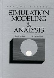
The definitive reference on discrete-event simulation; reading it here teaches rigorous model validation, output analysis, and statistical credibility — critical skills before tackling stochastic advanced topics.
Stochastic & Optimization-Based Modeling
ExpertBuild and analyze models that incorporate uncertainty, randomness, and optimal decision-making — the frontier of applied mathematical modeling in science, engineering, and economics.
▸ Study plan for this stage
Pace: 8–10 weeks, ~40–50 pages/day (Taylor first 3–4 weeks, Williams 4–5 weeks, with 1–2 weeks for integration and projects)
- Stochastic processes (Markov chains, Poisson processes, random walks) and their role in modeling systems with randomness and memory
- Probability distributions, transition matrices, and steady-state analysis for predicting long-term system behavior
- Mathematical programming formulations: decision variables, objective functions, and constraints in linear, integer, and nonlinear optimization
- Uncertainty quantification and sensitivity analysis—how to incorporate randomness into deterministic optimization models
- Coupling stochastic and optimization frameworks: stochastic programming, expected value models, and robust optimization under uncertainty
- Real-world application domains: queueing systems, inventory management, resource allocation, and financial risk modeling
- Computational methods for solving large-scale stochastic and optimization problems, including simulation and approximation techniques
- What is a Markov chain, and how do transition probabilities determine the long-term behavior of a stochastic system?
- How would you formulate a linear programming problem for a resource allocation decision, and what role do constraints play?
- What is the difference between a deterministic optimization model and a stochastic programming model, and when should you use each?
- How can you use steady-state analysis from stochastic modeling to inform optimal decision-making in a queuing or inventory system?
- What are the main challenges in solving large-scale stochastic optimization problems, and what computational approaches does Williams discuss?
- How would you design a sensitivity analysis to test how uncertainty in input parameters affects an optimal solution?
- Build a Markov chain model for a simple system (e.g., weather states, customer loyalty, equipment failure) and compute its steady-state distribution by hand and computationally
- Formulate and solve a linear programming problem from a real-world scenario (e.g., production planning, diet optimization) using a solver (Python/PuLP, Excel Solver, or CPLEX)
- Model a queueing system (M/M/1 or M/M/c) using stochastic processes from Taylor, then optimize staffing or service capacity using programming techniques from Williams
- Create a two-stage stochastic programming model (e.g., inventory or investment problem) where first-stage decisions are made before uncertainty is revealed, and second-stage recourse actions follow
- Implement a Monte Carlo simulation to estimate the expected cost or profit of a decision under uncertainty, then compare against a deterministic optimization baseline
- Conduct a sensitivity analysis on a linear or integer programming model: vary key parameters (costs, demands, capacities) and visualize how the optimal solution changes
Next up: This stage equips you with the mathematical and computational foundations to model complex, uncertain, real-world systems and optimize decisions within them—preparing you to tackle specialized advanced topics such as dynamic programming, Markov decision processes, reinforcement learning, or domain-specific applications (e.g., supply chain optimization, financial engineering, or climate/environment
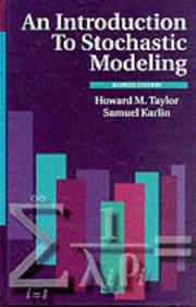
Develops Markov chains, Poisson processes, and stochastic differential equations as modeling tools; its applied orientation makes it the natural first step into probabilistic modeling after the deterministic stages.

Focuses entirely on the craft of formulating real-world optimization problems as mathematical programs; it rounds out the curriculum by adding the decision-making dimension that pure dynamical or stochastic models lack.
Discussion
Keep reading
Paths that share books, cover the same subject, or open a related topic.