The Best Books on Control Systems Engineering, In Order
This curriculum is designed for expert-level engineers who already possess strong mathematical foundations and want to achieve deep, research-grade mastery of control systems — from rigorous classical and state-space theory through nonlinear dynamics, optimal control, and robust/modern synthesis. Each stage sharpens a distinct layer of understanding, with books ordered so that notation, vocabulary, and intuitions introduced early are immediately leveraged in later texts.
Classical & State-Space Foundations (Expert Refresh)
ExpertSolidify rigorous command of frequency-domain methods, state-space representation, controllability/observability, and stability — the shared language all later texts assume.
▸ Study plan for this stage
Pace: 12–14 weeks, ~40–50 pages/day (mix of theory, derivations, and worked examples). Ogata: 5–6 weeks; D'Azzo: 4–5 weeks; Kailath: 3–4 weeks.
- Frequency-domain representation: transfer functions, poles, zeros, and their geometric interpretation in the s-plane; Bode, Nyquist, and Nichols plots as tools for stability and performance analysis
- State-space formulation: canonical forms (controllable, observable, diagonal, Jordan), state-feedback design, and observer construction; equivalence between transfer-function and state-space descriptions
- Controllability and observability: Kalman rank conditions, physical interpretation, and implications for system design and sensor/actuator placement
- Stability analysis: Routh–Hurwitz criterion, Lyapunov methods (direct and indirect), and frequency-domain stability margins (gain and phase margins)
- System interconnection and block-diagram algebra: cascade, parallel, and feedback configurations; signal-flow graphs and Mason's gain formula
- Transient and steady-state response: time-domain specifications (rise time, settling time, overshoot), relationship to pole location and frequency response
- Linear matrix inequalities (LMI) and quadratic forms: foundation for modern robust and optimal control formulations
- Minimal realization and system identification: connection between input–output behavior and internal state structure
- Given a transfer function, sketch its Bode and Nyquist plots by hand; identify gain and phase margins; determine closed-loop stability using the Nyquist criterion.
- Convert a transfer function to state-space form (multiple canonical forms); verify controllability and observability; explain what uncontrollable or unobservable modes mean physically.
- Design a state-feedback gain K to place closed-loop poles at desired locations; construct a full-state observer and verify its eigenvalues; combine them into a compensator.
- Apply Lyapunov's direct method to prove stability of a nonlinear or time-varying system; construct a Lyapunov function and verify conditions analytically.
- Analyze a multi-input, multi-output (MIMO) system: determine its rank, minimal realization, and structural properties (controllability, observability) using Kalman decomposition.
- Relate frequency-domain specifications (bandwidth, resonance peak) to time-domain step-response metrics (overshoot, settling time) and pole locations in the complex plane.
- Ogata Ch. 2–3: Solve 5–8 transfer-function problems (finding poles/zeros, sketching root locus); verify answers using MATLAB/Python (Control Systems Toolbox or python-control).
- Ogata Ch. 4–5: Construct Bode and Nyquist plots for 4–6 systems (low-order, then with time delays); measure gain and phase margins; predict closed-loop stability.
- Ogata Ch. 6–7: Convert 3–4 transfer functions to state-space; verify controllability and observability using rank tests; identify and interpret uncontrollable/unobservable modes.
- D'Azzo Ch. 3–4: Design state-feedback gains for 2–3 systems using pole-placement; simulate closed-loop step response and compare to specifications.
- D'Azzo Ch. 5–6: Build full-state observers for 2–3 systems; combine observer with state-feedback to form a compensator; simulate and verify observer convergence.
- Kailath Ch. 1–2: Prove controllability and observability for 2–3 MIMO systems using Kalman rank conditions; perform minimal realization and verify equivalence.
Next up: This stage establishes the mathematical and conceptual bedrock—transfer functions, state-space models, stability criteria, and structural properties—that all subsequent advanced topics (robust control, optimal control, adaptive systems, nonlinear analysis) depend on and extend.
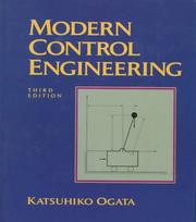
The definitive classical reference for transfer functions, root locus, Bode/Nyquist, and PID design. Reading it first at expert level enforces precise vocabulary and exposes any gaps before moving to state-space depth.
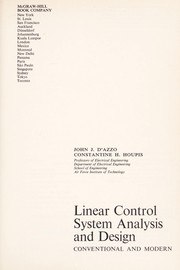
Bridges classical frequency-domain and modern state-space perspectives with rigorous treatment of stability criteria, making it the ideal transition text before pure state-space books.
The authoritative graduate-level treatment of linear system theory — realization, canonical forms, and algebraic structure — providing the mathematical bedrock for every advanced topic that follows.
Optimal & Multivariable Control
ExpertMaster LQR/LQG design, Kalman filtering, and MIMO control synthesis, understanding the optimization principles that underpin modern controller design.
▸ Study plan for this stage
Pace: 8–10 weeks, ~40–50 pages/day (Stengel first 4–5 weeks, Maciejowski next 4–5 weeks)
- Optimal control formulation: cost functions, performance indices, and the principle of optimality underlying dynamic programming
- Linear Quadratic Regulator (LQR): derivation via calculus of variations, Riccati equation solution, and closed-loop gain interpretation
- Kalman filtering: state estimation from noisy measurements, the innovation process, and duality between LQR and Kalman filter
- Linear Quadratic Gaussian (LQG) control: separation principle, combined estimation and control, and robustness limitations
- MIMO system representation: state-space models, controllability/observability, and pole placement in multivariable systems
- Multivariable feedback design: interaction analysis, decoupling strategies, and trade-offs between performance and robustness
- Nyquist and frequency-domain methods for MIMO systems: singular value analysis and robust stability margins
- Practical design constraints: actuator saturation, measurement noise, and implementation considerations in real systems
- Derive the LQR gain matrix from first principles using the Riccati equation, and explain how the weighting matrices Q and R shape the closed-loop response
- What is the duality between the LQR problem and Kalman filtering, and how does the separation principle justify using an LQG controller?
- Given a MIMO system with known disturbances and measurement noise, design a Kalman filter to estimate the full state and explain the role of process and measurement noise covariances
- Compare decoupling and non-decoupling approaches to MIMO control design; when is each appropriate, and what are the trade-offs?
- Analyze the robustness of an LQG controller using singular value plots; why is LQG less robust than classical methods, and how can you mitigate this?
- Design an LQR controller for a 2×2 MIMO system (e.g., aircraft lateral-directional dynamics) and validate stability, performance, and actuator constraints
- Work through Stengel's derivation of the Riccati equation (Chapter 4) by hand; solve a 2×2 system numerically and plot the closed-loop poles as Q/R ratios vary
- Implement a discrete-time Kalman filter in MATLAB/Python for a simple 2-state system with process and measurement noise; compare filter estimates to true state and validate convergence
- Design an LQR controller for a linearized inverted pendulum or aircraft model; tune Q and R matrices to achieve specified settling time and overshoot, then simulate closed-loop response
- Combine LQR and Kalman filter into an LQG controller for a system with full-state feedback unavailable; compare LQG performance to LQR with perfect state information
- Analyze a 2×2 or 3×3 MIMO system (e.g., distillation column, aircraft) using Maciejowski's methods: compute singular values, design a decoupling compensator, and assess interaction
- Perform a robustness analysis on an LQG design using Nyquist plots and singular value margins; identify gain and phase margins and propose modifications to improve robustness
Next up: This stage equips you with optimization-based design tools and robustness analysis methods that form the foundation for advanced topics such as H∞ control, μ-synthesis, and adaptive/nonlinear control, where you will extend these principles to handle uncertainty and time-varying systems.
Covers LQR, LQG, and Kalman filtering in a unified, application-grounded framework; its accessible derivations build strong intuition before the more abstract treatments ahead.

Provides rigorous MIMO design methodology — singular values, loop shaping, and H∞ precursors — directly extending LQG intuition into multivariable frequency-domain thinking.
Robust Control & H∞ Synthesis
ExpertAchieve deep understanding of uncertainty modeling, robust stability, H∞ and H₂ optimal synthesis, and structured singular value (μ) analysis.
▸ Study plan for this stage
Pace: 8–10 weeks, ~40–50 pages/day with 2–3 days/week dedicated to problem-solving and simulations
- Uncertainty modeling: unstructured perturbations (additive, multiplicative, feedback) and structured uncertainty (parametric, block-diagonal)
- Robust stability: small-gain theorem, structured singular value (μ) as a tool for analyzing robustness to structured uncertainty
- H∞ norm: definition, computation, and interpretation as the peak gain across frequencies; connection to worst-case disturbance rejection
- H∞ synthesis: formulation of weighted sensitivity/complementary sensitivity problems and solution via Riccati equations and state-space algorithms
- H₂ optimal control: LQR framework, Wiener filtering, and comparison with H∞ approaches for different design objectives
- μ-synthesis and D-K iteration: iterative design loop for structured uncertainty using scaling and controller refinement
- Practical robustness metrics: gain margin, phase margin, and their relationship to multiplicative uncertainty bounds
- Trade-offs in robust design: balancing nominal performance, robust stability, and computational complexity
- How do unstructured and structured uncertainty models differ, and when is each appropriate for a given control problem?
- Explain the small-gain theorem and how it underpins robust stability analysis; what role does the structured singular value play?
- Define the H∞ norm of a transfer function and describe how it relates to the maximum singular value across the frequency spectrum.
- Walk through the standard H∞ synthesis problem: how are performance and robustness objectives encoded in weighted sensitivity functions, and what does the solution controller achieve?
- Compare H∞ and H₂ optimal control: what are the design objectives, solution methods, and practical trade-offs of each?
- What is the D-K iteration in μ-synthesis, and why is it necessary for controller design under structured uncertainty?
- How do classical margins (gain and phase) relate to multiplicative uncertainty bounds, and what are their limitations in robust design?
- Construct additive, multiplicative, and feedback uncertainty models for a given nominal plant; compute and compare their robust stability margins using the small-gain theorem.
- Compute the H∞ norm of 3–4 transfer functions by hand (pole-residue analysis or frequency sweep) and verify using MATLAB/Python (Control Systems Toolbox or similar).
- Formulate a weighted sensitivity minimization problem for a benchmark system (e.g., mass-spring-damper or aircraft pitch control); solve using hinfsyn or equivalent and interpret the resulting controller.
- Implement H₂ optimal control (LQR) for the same benchmark system; compare the closed-loop H∞ norm, H₂ norm, and step response with the H∞ design.
- Perform μ-analysis on a 2×2 or 3×3 uncertain system using structured singular value tools; identify the frequency range and uncertainty direction most threatening to stability.
- Execute one complete D-K iteration cycle: scale the uncertainty, design a controller, compute μ, refine scaling, and iterate until convergence; document improvements in robustness margin.
- Analyze a real or realistic control problem (e.g., flexible beam, magnetic levitation, or aircraft control) using both classical margins and H∞/μ-based robustness metrics; discuss discrepancies and design trade-offs.
- Reproduce a case study or numerical example from Zhou's texts (e.g., a benchmark problem in Chapter 5 or 6 of *Robust and Optimal Control*); extend it by adding structured uncertainty or tightening performance specs.
Next up: This stage equips you with the mathematical and computational tools to design controllers that maintain stability and performance despite model uncertainty; the next stage will likely focus on applying these techniques to multivariable systems, nonlinear robustness, or real-world implementation challenges such as computational constraints and sensor/actuator limitations.

The canonical graduate text for H∞ theory, presenting Riccati-equation and LMI-based synthesis with full mathematical rigor — the standard reference in robust control research.

A focused distillation of the same author's comprehensive work, ideal for consolidating core robust control concepts and μ-synthesis before tackling nonlinear and geometric methods.
Nonlinear Dynamics & Control
ExpertDevelop rigorous tools for analyzing and controlling nonlinear systems: Lyapunov stability, feedback linearization, sliding mode, and passivity-based control.
▸ Study plan for this stage
Pace: 12–14 weeks, ~40–50 pages/day. Strogatz (Weeks 1–5, ~350 pages); Khalil (Weeks 6–14, ~550 pages). Allocate 1–2 days per chapter for deep study and problem-solving.
- Phase portraits, fixed points, and linearization: understanding local behavior of nonlinear systems through geometric visualization and Jacobian analysis
- Lyapunov stability theory: constructing Lyapunov functions to prove global/local stability without solving differential equations
- Bifurcations and their types (saddle-node, transcritical, pitchfork, Hopf): recognizing how system qualitative behavior changes with parameters
- Limit cycles, periodic orbits, and attractors: identifying and analyzing self-sustained oscillations in nonlinear systems
- Feedback linearization: transforming nonlinear systems into linear ones via state feedback and coordinate changes for control design
- Sliding mode control: designing robust controllers that force trajectories onto a sliding surface for finite-time convergence
- Passivity and dissipativity: using energy-based methods to guarantee stability and design controllers for complex nonlinear systems
- Input-to-state stability (ISS) and robustness: analyzing how bounded disturbances affect nonlinear system behavior
- How do you construct a phase portrait for a 2D nonlinear system, and what do fixed points, separatrices, and limit cycles tell you about long-term behavior?
- Explain the Lyapunov direct method: how do you construct a Lyapunov function, and why does V̇ ≤ 0 guarantee stability without solving the system?
- What is a bifurcation, and how do saddle-node, transcritical, pitchfork, and Hopf bifurcations differ geometrically and in their control implications?
- Describe feedback linearization: when is it applicable, what is the relative degree, and how do you design a control law to achieve desired closed-loop dynamics?
- How does sliding mode control work, and why does it provide robustness to matched disturbances and parameter uncertainty?
- Define passivity and dissipativity. How can you use passivity-based control to stabilize a nonlinear system, and what are the advantages over classical feedback?
- What is input-to-state stability (ISS), and how does it extend Lyapunov stability to systems with disturbances?
- Strogatz Ch. 2–3: Sketch phase portraits for 5–10 canonical systems (logistic map, pendulum, van der Pol oscillator, Lorenz system). Identify fixed points, stability via eigenvalues, and separatrices by hand.
- Strogatz Ch. 4–5: Perform bifurcation analysis on 3 parameter-dependent systems (e.g., ẋ = r + x − x³). Plot bifurcation diagrams and explain the transition in qualitative behavior.
- Khalil Ch. 3–4: Construct Lyapunov functions for 4–6 nonlinear systems using standard forms (quadratic, sum-of-squares). Verify V̇ ≤ 0 and determine stability regions.
- Khalil Ch. 5: Apply feedback linearization to 2–3 systems (e.g., magnetic levitation, inverted pendulum). Compute relative degree, design state feedback, and simulate closed-loop response.
- Khalil Ch. 6: Design a sliding mode controller for a 2nd-order nonlinear system. Prove finite-time convergence and test robustness to ±20% parameter variations via simulation.
- Khalil Ch. 8–9: Analyze passivity of 2–3 nonlinear systems. Design a passivity-based controller and compare stability margins with classical PID on a benchmark problem (e.g., robot manipulator).
Next up: Mastery of Lyapunov stability, feedback linearization, sliding mode, and passivity-based control provides the theoretical foundation and design tools needed for advanced topics such as adaptive control, robust control synthesis, and nonlinear observer design in subsequent stages.
Builds deep geometric and qualitative intuition for nonlinear behavior — bifurcations, limit cycles, chaos — that is essential context before tackling formal nonlinear control synthesis.
The definitive graduate text on nonlinear control: Lyapunov methods, input-output stability, feedback linearization, and backstepping, presented with full mathematical rigor.
Complements Khalil with an engineering-oriented treatment of sliding mode control, adaptive control, and robot dynamics, grounding abstract theory in concrete design procedures.
Advanced Topics: Geometric, Adaptive & Data-Driven Control
ExpertReach the research frontier — geometric control on manifolds, model-reference adaptive systems, and modern data-driven/learning-based control paradigms.
▸ Study plan for this stage
Pace: 12–14 weeks, ~40–50 pages/day (alternating focus: 2–3 weeks on Murray's geometric foundations, then 3–4 weeks on Åström's adaptive control theory, then 2–3 weeks integrating both with applications, then 2–3 weeks on advanced topics and research papers)
- Lie groups and Lie algebras as configuration spaces for robotic systems; exponential coordinates and their role in geometric control
- Differential geometry on manifolds: tangent spaces, vector fields, Lie brackets, and their control-theoretic interpretation
- Controllability and accessibility on manifolds; Lie algebra rank condition and its geometric meaning
- Nonlinear control design via feedback linearization, input-output linearization, and geometric control laws
- Model-reference adaptive control (MRAC): reference models, adaptive laws, and stability via Lyapunov theory
- Parameter estimation and persistent excitation; convergence conditions for adaptive systems
- Robustness of adaptive control; handling unmodeled dynamics and disturbances
- Data-driven and learning-based control paradigms: neural networks, reinforcement learning, and their integration with classical adaptive control
- How do Lie groups and exponential coordinates provide a natural framework for representing rigid-body configurations, and why is this superior to Euler angles for control design?
- What is the Lie algebra rank condition (LARC) and how does it generalize controllability from linear systems to nonlinear systems on manifolds?
- Explain the difference between input-output linearization and full state feedback linearization; when would you use each?
- In model-reference adaptive control, what role does persistent excitation play in ensuring parameter convergence, and what happens without it?
- How do modern data-driven control methods (e.g., neural network-based policies) differ from classical adaptive control in their assumptions and guarantees?
- Design an adaptive control law for a nonlinear system with unknown parameters; justify your choice of adaptation rule and Lyapunov function.
- Work through Murray's examples on SE(3) and SO(3): compute Lie brackets, verify the Lie algebra rank condition for a 3-DOF manipulator, and sketch the reachable set
- Implement feedback linearization for a 2-DOF planar manipulator using Murray's formulation; simulate tracking a desired trajectory and compare with PID control
- Derive and simulate a model-reference adaptive controller for a first-order system with unknown gain (Åström's canonical example); plot parameter convergence and tracking error over time
- Extend the adaptive controller to a second-order system (e.g., mass-spring-damper with unknown mass); verify stability using the Lyapunov function from Åström's theory
- Analyze a nonlinear system (e.g., inverted pendulum) for controllability using the Lie algebra rank condition; design a geometric control law and compare with classical nonlinear methods
- Implement a simple neural network-based adaptive controller for a nonlinear system; compare convergence speed, robustness, and parameter interpretability with classical MRAC
Next up: This stage establishes the mathematical foundations (geometric control on manifolds) and classical adaptive paradigms (MRAC, parameter estimation) that underpin modern research in learning-based control, robust adaptive systems, and autonomous decision-making—preparing you to engage with current literature on neural-adaptive control, safe reinforcement learning, and data-driven optimization for co
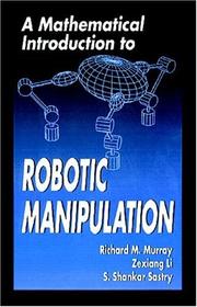
Introduces geometric (Lie group) control theory through the lens of robotics, extending classical state-space ideas to systems evolving on nonlinear manifolds.
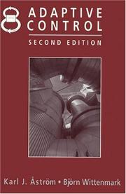
The authoritative text on model-reference and self-tuning adaptive control by one of its founders, providing both theory and practical design insight unavailable elsewhere.
Discussion
Keep reading
Paths that share books, cover the same subject, or open a related topic.