The Best Books to Learn Partial Differential Equations, In Order
This curriculum is designed for expert-level learners who already have strong mathematical maturity (real analysis, ODEs, linear algebra) and want to achieve deep mastery of PDEs — from rigorous classical theory through modern functional-analytic and nonlinear methods. The four stages move from systematic classical foundations, through Sobolev-space and variational theory, into advanced nonlinear and geometric PDEs, and finally into specialized research-level topics, ensuring each book builds directly on the language and results of its predecessors.
Classical Theory & Methods
BeginnerCommand the classical PDE toolkit — characteristics, separation of variables, Fourier methods, Green's functions, and the canonical equations (Laplace, heat, wave) — with rigorous proofs and physical intuition.
▸ Study plan for this stage
Pace: 12–14 weeks, ~40–50 pages/day (Evans: ~6 weeks; Strauss: ~6–8 weeks, with 1–2 weeks for integration and problem sets)
- Method of characteristics: solving first-order PDEs by reducing to ODEs along characteristic curves
- Separation of variables: decomposing multi-variable PDEs into products of single-variable ODEs
- Fourier series and Fourier transforms: representing solutions as superpositions of eigenfunctions
- The heat equation: parabolic PDE, maximum principle, fundamental solution, and well-posedness
- The wave equation: hyperbolic PDE, d'Alembert's formula, energy methods, and finite propagation speed
- Laplace's equation: elliptic PDE, harmonic functions, maximum principle, and regularity
- Green's functions: constructing solutions via integral representations and reciprocity
- Weak solutions and Sobolev spaces: rigorous foundations for existence and uniqueness (Evans focus)
- How does the method of characteristics reduce a first-order PDE to an ODE, and what does a characteristic curve represent geometrically?
- Explain separation of variables: why does assuming u(x,t) = X(x)T(t) work, and what boundary/initial conditions determine the separated ODEs?
- State the maximum principle for the heat equation and Laplace's equation. Why does it imply uniqueness of solutions?
- Derive or explain d'Alembert's formula for the wave equation on ℝ. What does it tell you about causality and domain of dependence?
- What is a Green's function, and how does it allow you to write solutions to inhomogeneous PDEs as integrals?
- Compare the three canonical equations (heat, wave, Laplace): which is parabolic/hyperbolic/elliptic, and what does this classification mean for well-posedness and solution regularity?
- Evans Ch. 2–3: Solve 5–8 first-order PDEs using characteristics (linear and quasi-linear cases); sketch characteristic curves for at least 2 problems.
- Evans Ch. 4: Apply separation of variables to the heat equation on [0,π] with Dirichlet BCs; compute the first 3–4 Fourier modes and plot the solution at t=0, t=0.1, t=1.
- Evans Ch. 4: Solve the wave equation on [0,1] with zero Dirichlet BCs and given initial displacement/velocity using separation of variables; verify energy conservation.
- Strauss Ch. 2–3: Solve 4–6 Laplace problems on rectangles, disks, and half-planes using separation of variables; verify harmonic property.
- Evans Ch. 5 or Strauss Ch. 4: Compute Green's functions for the Laplacian on simple domains (interval, disk); use them to solve an inhomogeneous Poisson problem.
- Strauss Ch. 1–2: Verify d'Alembert's formula for 2–3 wave equation problems; identify domain of dependence and check causality.
- Evans Ch. 5–6: Prove the maximum principle for the heat equation; apply it to show uniqueness for a non-trivial initial-boundary value problem.
- Mixed: Classify 8–10 given PDEs as parabolic/hyperbolic/elliptic and predict qualitative behavior (smoothing, finite speed, oscillation) before solving.
Next up: This stage equips you with the classical toolkit and physical intuition for canonical PDEs; the next stage will deepen your understanding through modern functional analysis (Sobolev spaces, weak formulations, and regularity theory) and extend to nonlinear PDEs and advanced techniques.

The gold-standard modern reference: Evans builds classical solutions (characteristics, fundamental solutions, mean-value formulas) with full rigor before introducing modern methods, making it the ideal anchor for the entire curriculum.

A concise, example-driven complement to Evans that sharpens intuition for the wave, heat, and Laplace equations through explicit solutions and physical interpretations before the abstraction deepens.
Functional Analysis & Sobolev Space Methods
IntermediateReformulate PDEs in weak/variational form, master Sobolev spaces and embedding theorems, and apply the Lax–Milgram theorem and elliptic regularity theory.
▸ Study plan for this stage
Pace: 8–10 weeks, ~40–50 pages/day (Brezis: Chapters 1–11, ~350 pages over 6–7 weeks; Gilbarg: Chapters 1–6, ~150 pages over 2–3 weeks)
- Weak derivatives and distributional derivatives: definition, properties, and how they generalize classical derivatives
- Sobolev spaces (W^{k,p}, H^k): construction, norms, completeness, and separability properties
- Sobolev embedding theorems: continuous and compact embeddings, critical exponents, and dimension-dependent behavior
- Weak formulation of PDEs: converting boundary value problems into variational equations and understanding solution existence
- Lax–Milgram theorem: conditions for unique solvability of coercive, continuous bilinear forms on Hilbert spaces
- Elliptic regularity theory: bootstrapping from weak to classical solutions, interior and boundary regularity
- Trace theorems and boundary conditions: rigorous treatment of Dirichlet and Neumann conditions in weak formulations
- Compact operators and spectral theory: eigenvalue problems for elliptic operators and Fredholm alternatives
- What is the difference between a classical derivative and a weak derivative, and why is the weak formulation necessary for PDEs with non-smooth data?
- State the definition of the Sobolev space W^{k,p}(Ω) and explain why it is a Banach space. What additional structure does H^k(Ω) have?
- Formulate the Dirichlet problem for the Poisson equation −Δu = f in weak form, and explain what it means for u to be a weak solution.
- State and apply the Lax–Milgram theorem: what conditions must a bilinear form satisfy, and what does the theorem guarantee?
- Explain the Sobolev embedding theorem in one dimension and higher dimensions. How does the critical exponent depend on dimension and regularity?
- What is elliptic regularity, and how does it allow you to conclude that a weak solution to an elliptic PDE is actually classical?
- Compute weak derivatives for non-smooth functions (e.g., |x|, |x|^α) and verify they satisfy the definition via integration by parts
- Prove that H^1(Ω) is a Hilbert space with the standard inner product and verify the Poincaré inequality for bounded domains
- Reformulate the Neumann problem −Δu + u = f with ∂u/∂n = g in weak form and identify the appropriate Sobolev space and boundary conditions
- Apply the Lax–Milgram theorem to prove existence and uniqueness of weak solutions to −Δu + cu = f with c > 0 on H^1_0(Ω)
- Verify Sobolev embedding: show that H^1(Ω) ⊂ L^4(Ω) in 2D and H^1(Ω) ⊂ C^0(Ω) in 1D using Morrey's inequality
- Work through a regularity bootstrap argument: assume u ∈ H^1 solves −Δu = f with f ∈ L^2, then show u ∈ H^2 and u ∈ C^∞ if f ∈ C^∞
Next up: This stage equips you with the variational machinery and regularity theory needed to analyze nonlinear PDEs, parabolic and hyperbolic equations, and numerical approximation schemes (finite element methods), where weak formulations and Sobolev space estimates are indispensable.
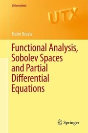
Brezis develops the functional-analytic machinery (Banach/Hilbert spaces, duality, compact operators) and Sobolev theory in tight coordination, providing exactly the tools needed for variational PDE theory.
The definitive deep dive into elliptic theory — maximum principles, Schauder estimates, and Calderón–Zygmund theory — read after Brezis to consolidate regularity theory at research depth.
Nonlinear PDEs & Advanced Analysis
ExpertUnderstand the analysis of nonlinear PDEs including viscosity solutions, conservation laws, Hamilton–Jacobi equations, and geometric measure-theoretic techniques.
▸ Study plan for this stage
Pace: 12–14 weeks, ~40–50 pages/day (with 2–3 days per week for problem-solving and reflection)
- Viscosity solutions: definition, existence, uniqueness, and comparison principles for nonlinear first-order PDEs
- Conservation laws: weak solutions, entropy conditions, and the role of shock waves in hyperbolic systems
- Hamilton–Jacobi equations: level set methods, reachability analysis, and connections to optimal control
- Shock formation and propagation: Rankine–Hugoniot conditions, entropy inequalities, and admissibility criteria
- Geometric measure theory in PDEs: rectifiable sets, varifolds, and mean curvature flow as a geometric PDE
- Nonlinear elliptic and parabolic equations: monotonicity methods, a priori estimates, and regularity theory
- Blow-up phenomena and finite-time singularities in nonlinear evolution equations
- Multivalued analysis and subdifferential calculus for nonsmooth nonlinear problems
- What is a viscosity solution, and why is this concept necessary for nonlinear first-order PDEs that lack classical solutions?
- State and explain the Rankine–Hugoniot jump condition and the entropy condition for admissible shocks in conservation laws.
- How do Hamilton–Jacobi equations relate to optimal control problems, and what role do viscosity solutions play in this connection?
- Describe the geometric measure-theoretic approach to mean curvature flow and explain how it handles singularities.
- What are the key differences between weak solutions and entropy solutions for hyperbolic conservation laws, and when is entropy selection necessary?
- Explain the comparison principle for viscosity solutions and its role in proving uniqueness.
- Work through Giga's examples of viscosity solutions for the eikonal equation |∇u| = 1 and verify the comparison principle directly.
- Solve Riemann problems for scalar conservation laws (e.g., Burgers' equation) and classify solutions as rarefaction waves, shocks, or contact discontinuities using entropy conditions.
- Derive the Rankine–Hugoniot condition from first principles using integral formulations and apply it to specific hyperbolic systems from Lax's text.
- Implement a numerical scheme (e.g., Godunov or Lax–Friedrichs) for a scalar conservation law and verify convergence to the entropy solution.
- Analyze a Hamilton–Jacobi equation arising from an optimal control problem: set up the equation, find the viscosity solution, and interpret it geometrically.
- Study a geometric PDE (e.g., mean curvature flow) from Jost's treatment and work through the existence and regularity theory for weak solutions.
Next up: This stage equips you with the analytical and geometric tools to handle singularities, weak solutions, and nonsmooth phenomena in PDEs, preparing you for specialized topics such as free boundary problems, variational methods in geometric analysis, or applications to nonlinear diffusion and pattern formation.

Provides a rigorous modern treatment of viscosity solutions and level-set methods, bridging the gap between classical/Sobolev theory and contemporary nonlinear analysis.
Lax's landmark monograph on hyperbolic conservation laws and shock theory is indispensable for understanding nonlinear wave phenomena and entropy conditions at the highest level.
Jost integrates geometric and analytic viewpoints — including harmonic maps and geometric flows — providing a bridge to the most modern research directions after the nonlinear foundations are set.
Microlocal Analysis & Spectral Theory
ExpertAchieve research-level command of pseudodifferential operators, microlocal analysis, and spectral theory of elliptic operators — the language of the modern PDE literature.
▸ Study plan for this stage
Pace: 12–16 weeks, ~40–50 pages/day (Hörmander I: weeks 1–10; Davies: weeks 11–16). Hörmander is dense; expect 2–3 readings per section. Davies is more applied; read faster but work through all proofs.
- Pseudodifferential operators: symbol classes, composition, asymptotic expansions, and the symbolic calculus that makes them a functional algebra
- Microlocal analysis: wavefront sets, characteristic sets, and how singularities propagate along bicharacteristics
- Elliptic regularity and hypoellipticity: when solutions inherit smoothness from data, and the role of the principal symbol
- Spectral theory of self-adjoint operators: spectrum, resolvent, spectral measures, and functional calculus
- Essential spectrum vs. discrete spectrum: Weyl's criterion and perturbation theory for elliptic operators
- Asymptotic distribution of eigenvalues: Weyl's law and heat kernel asymptotics
- Fredholm theory and index: how pseudodifferential operators define Fredholm operators and topological invariants
- What is a symbol of order m, and how do you compose two pseudodifferential operators to get an asymptotic expansion of the product symbol?
- Define the wavefront set of a distribution and explain why it is invariant under smooth changes of variables.
- State and prove the elliptic regularity theorem: if P is elliptic and Pu ∈ H^s, what can you conclude about u?
- For a self-adjoint elliptic operator on a compact manifold, distinguish between the discrete spectrum and essential spectrum, and state Weyl's criterion.
- Explain Weyl's law: what does it say about the asymptotic growth of eigenvalues, and why is it important for understanding the spectrum?
- What is the index of a Fredholm pseudodifferential operator, and how does it relate to the winding number of the principal symbol?
- Compute the symbol of the product of two pseudodifferential operators of orders m₁ and m₂; verify the first two terms of the asymptotic expansion by hand for a concrete example (e.g., Δ ∘ ∂ₓ on ℝ).
- For the Laplacian on the circle S¹, compute the wavefront set of a distribution with a jump discontinuity; verify that it lies in the characteristic set.
- Prove elliptic regularity for a second-order elliptic operator in divergence form on ℝⁿ using energy estimates and Fourier analysis.
- For the Dirichlet Laplacian on a bounded domain Ω ⊂ ℝⁿ, compute the first 5–10 eigenvalues numerically and compare with Weyl's law asymptotics.
- Construct the spectral measure for the operator d²/dx² on L²(ℝ) with appropriate boundary conditions; compute ∫ λ dE(λ) for a test function.
- Show that the essential spectrum of a Schrödinger operator −Δ + V on ℝⁿ equals [0, ∞) when V → 0 at infinity, using Weyl's criterion.
- Compute the index of a first-order elliptic pseudodifferential operator on S¹ by analyzing the winding number of its principal symbol.
- Work through a complete proof of the heat kernel asymptotics for an elliptic operator; extract the leading coefficient and relate it to the volume.
Next up: Mastery of pseudodifferential operators and spectral theory provides the technical foundation for analyzing nonlinear PDEs, geometric analysis, and inverse problems — the next stage will apply these tools to understand how singularities and spectra behave under nonlinear perturbations and in inverse scattering.
Hörmander's four-volume treatise is the definitive reference for distribution theory and microlocal analysis; Volume I on distribution theory and Fourier analysis is the essential entry point to this stage.

Davies provides a rigorous and accessible account of spectral theory for differential operators in Hilbert space, completing the curriculum with the tools needed to read current research papers on PDEs.
Discussion
Keep reading
Paths that share books, cover the same subject, or open a related topic.