The Best Books to Learn Bayesian Statistics, In Order
This curriculum builds a deep, rigorous understanding of Bayesian statistics across four progressive stages. Starting from intermediate-level probability, it moves through core Bayesian inference, probabilistic modeling, and finally advanced computational and theoretical methods — each stage equipping the reader with the vocabulary and intuition needed for the next.
Foundations & Intuition
BeginnerReframe probability as a measure of belief, understand Bayes' theorem deeply, and build the intuitive scaffolding needed for formal Bayesian reasoning.
▸ Study plan for this stage
Pace: 6–8 weeks, ~25–30 pages/day (alternating between both books; ~2 weeks per book, with 1–2 weeks for integration and practice)
- Probability as a measure of subjective belief, not just frequency—how prior beliefs get updated by evidence
- Bayes' theorem as a formal rule for updating beliefs: P(H|D) = P(D|H)P(H) / P(D), and why each component matters
- Prior, likelihood, and posterior: how to identify and reason about each in a real problem
- The mechanics of Bayesian updating: how new data shifts your credence in a hypothesis
- Grid approximation and simple computational methods for solving Bayes' theorem without calculus
- Common pitfalls: base rate neglect, misinterpreting probability, and how Bayesian thinking avoids them
- Building intuition through concrete, relatable examples (medical tests, coin flips, detective work) before abstraction
- What is the difference between frequentist and Bayesian interpretations of probability, and why does the Bayesian view treat probability as a degree of belief?
- State Bayes' theorem and explain what each term (prior, likelihood, posterior, evidence) represents in a concrete example like a medical diagnosis or spam detection.
- Given a real-world scenario (e.g., 'You observe a positive test result for a rare disease'), walk through the step-by-step process of updating your belief using Bayes' theorem.
- How does the prior belief influence the posterior? What happens if you start with a very strong prior versus a weak one?
- Explain grid approximation: how would you use it to solve a Bayesian problem computationally, and why is it useful for building intuition?
- Identify the base rate fallacy in a given scenario and explain how Bayesian reasoning corrects for it.
- Work through 'Bayesian Statistics the Fun Way' Chapter 2–3 exercises: calculate posterior probabilities for simple scenarios (coin flips, disease tests) by hand using Bayes' theorem.
- Implement grid approximation in Python or R for a simple problem (e.g., estimating the bias of a coin given observed flips). Plot the prior, likelihood, and posterior to visualize the update.
- Solve the 'Cookie Problem' and 'Monty Hall' problem from 'Think Bayes' using both intuitive reasoning and Bayes' theorem; compare your answers.
- Create a 'belief update journal': pick 3 real-world beliefs you hold (e.g., 'This person is trustworthy', 'It will rain tomorrow'). For each, identify what prior you started with and what evidence would update it; calculate the posterior for one using Bayes' theorem.
- Replicate one of the worked examples from 'Think Bayes' (e.g., the locomotive problem or the Dungeons & Dragons dice problem) in code, then modify the prior or data and observe how the posterior changes.
- Write a 1–2 page explanation of a real-world Bayesian reasoning scenario (medical diagnosis, legal evidence, product quality control) that clearly identifies the prior, likelihood, and posterior, and explains why ignoring the prior would be a mistake.
Next up: This stage builds the conceptual and computational foundation—understanding *why* Bayes' theorem works and *how* to apply it to simple problems—which prepares you to tackle more complex models, distributions, and inference techniques in the next stage (e.g., conjugate priors, MCMC, hierarchical models).

A highly accessible, example-driven introduction that builds genuine intuition for priors, likelihoods, and posteriors without heavy math — ideal for resetting intuitions before going deeper.
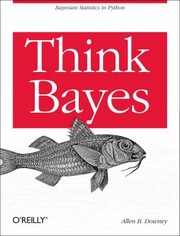
Reinforces Bayesian thinking through computational examples in Python, bridging intuition and implementation and preparing the reader for more formal treatments.
Core Bayesian Inference
IntermediateMaster the mechanics of Bayesian inference — conjugate priors, posterior distributions, credible intervals, and model comparison — with mathematical rigor.
▸ Study plan for this stage
Pace: 8–10 weeks, ~40–50 pages/day (mix of reading and worked examples). Kruschke: weeks 1–5 (~300 pages); Gelman: weeks 6–10 (~400 pages). Allocate 2–3 days per major chapter for re-reading and note-taking.
- Bayes' theorem as the foundation: P(θ|data) ∝ P(data|θ)P(θ), and how prior, likelihood, and posterior relate
- Conjugate priors (Beta-Binomial, Normal-Normal, Gamma-Poisson) and why they enable closed-form posteriors
- Posterior distributions as complete summaries of uncertainty: extracting point estimates, credible intervals, and predictive distributions
- Markov Chain Monte Carlo (MCMC) methods—Metropolis-Hastings and Gibbs sampling—for approximating posteriors when conjugacy fails
- Model comparison via Bayes factors and posterior predictive checks: quantifying evidence for competing hypotheses
- Hierarchical models and multilevel thinking: pooling information across groups and managing uncertainty at multiple levels
- Practical workflow: prior specification, sensitivity analysis, convergence diagnostics (Rhat, effective sample size), and posterior predictive simulation
- Derive the posterior distribution for a Beta-Binomial model: given a Beta(α, β) prior and n Bernoulli trials with k successes, what is P(θ|data)?
- Explain why conjugate priors are computationally convenient and give two examples from Kruschke's work; when would you *not* use them?
- What is a credible interval, how does it differ from a frequentist confidence interval, and how do you extract one from a posterior sample?
- Describe the Metropolis-Hastings algorithm: what is the acceptance ratio, why is it necessary, and what can go wrong if the proposal distribution is poorly tuned?
- How do you use posterior predictive checks to assess model fit? Why is comparing observed data to replicated data under the posterior more informative than point estimates alone?
- Define a Bayes factor; how would you compute one for two competing models, and what does a Bayes factor of 10 mean in plain language?
- Work through Kruschke's Beta-Binomial coin-flip example (Ch. 5–6) by hand: compute the posterior analytically, then verify with a grid approximation and MCMC. Plot prior, likelihood, and posterior on the same graph.
- Implement a Metropolis-Hastings sampler from scratch (in R or Python) for a simple 1D problem (e.g., estimating μ in a Normal model with unknown σ). Diagnose convergence using trace plots and Rhat; explain what you see.
- Replicate one of Gelman's hierarchical examples (e.g., the eight schools problem or radon data): fit the model, extract posterior summaries, and interpret the pooling of information across groups.
- Conduct a prior sensitivity analysis: fit a Bayesian model with three different priors (weak, moderate, strong) and compare posterior distributions. Document how much the choice of prior matters.
- Perform a posterior predictive check: simulate replicated datasets under the posterior and compare a test statistic (e.g., mean, max) to the observed data. Interpret whether the model captures key features.
- Compare two competing models using Bayes factors or leave-one-out cross-validation (LOO-IC from Gelman). Interpret the evidence for each model and discuss practical implications.
Next up: This stage equips you with the mathematical and computational foundations of Bayesian inference; the next stage will extend these tools to modern applications—advanced hierarchical models, causal inference, and domain-specific workflows—building on your fluency with posteriors, MCMC, and model comparison.

Known as the 'Puppy Book,' it provides a thorough, mathematically honest treatment of Bayesian inference with worked examples, making it the ideal first rigorous text.
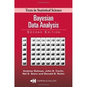
The definitive reference for Bayesian inference and modeling; reading it after Kruschke ensures the reader can absorb its depth and use it as a long-term reference.
Probabilistic Modeling & Programming
IntermediateLearn to build, specify, and fit hierarchical and probabilistic models using modern probabilistic programming tools, and understand the modeling workflow end-to-end.
▸ Study plan for this stage
Pace: 12–14 weeks, ~40–50 pages/day (Statistical Rethinking: 6–7 weeks, ~35 pages/day; Bayesian Modeling and Computation in Python: 6–7 weeks, ~45 pages/day)
- Generative modeling: thinking of data as arising from a process, and building models that reflect that process
- Hierarchical models: pooling information across groups using multilevel structures to handle varying intercepts and slopes
- Posterior inference: using Markov Chain Monte Carlo (MCMC) and variational inference to approximate posterior distributions
- Model specification and DAGs: using directed acyclic graphs to clarify causal assumptions and dependencies in probabilistic models
- Probabilistic programming: writing models as code using tools like Stan (via pymc) and PyMC to automate inference
- Prior specification and sensitivity: choosing priors thoughtfully, understanding their impact, and conducting prior predictive checks
- Posterior predictive checks and model criticism: validating models by simulating from the posterior and comparing to observed data
- Workflow integration: moving fluidly from question formulation through model building, fitting, diagnostics, and interpretation
- What is a generative model, and how does thinking generatively change the way you approach a statistical problem?
- How do hierarchical (multilevel) models improve inference when you have data grouped by categories, and what is the advantage of partial pooling?
- How do you specify a probabilistic model using a DAG, and what role do causal assumptions play in model design?
- What is the difference between prior predictive checks and posterior predictive checks, and when would you use each?
- How do you translate a mathematical model specification into probabilistic programming code (e.g., in PyMC), and what does the sampler do?
- What are common MCMC diagnostics (trace plots, R-hat, effective sample size), and how do you interpret them to assess convergence?
- Work through Statistical Rethinking's code examples (Chapters 4–9) in R or Python, reproducing plots and posterior summaries for linear, generalized linear, and multilevel models.
- Build a simple hierarchical model from scratch: specify the generative process, draw a DAG, write the prior and likelihood, and fit it using PyMC to real grouped data (e.g., school performance, patient outcomes across clinics).
- Conduct a prior predictive check: simulate data from your priors before fitting, visualize the implied predictions, and adjust priors if they are unreasonable.
- Fit a multilevel regression to a dataset with varying intercepts and slopes (e.g., Radon levels by county, or student test scores by school); compare results to a pooled and unpooled model.
- Perform posterior predictive checks on a fitted model: generate replicated datasets from the posterior, compute test statistics, and compare to the observed data to identify model misfit.
- Diagnose MCMC convergence: examine trace plots, compute R-hat and effective sample size, and adjust sampler settings (chains, tuning, target acceptance rate) to improve diagnostics.
Next up: Mastering the end-to-end workflow of model specification, fitting, and criticism positions you to tackle advanced topics such as causal inference, model comparison, and specialized model families (time series, spatial models, Gaussian processes) in the next stage.

Teaches Bayesian modeling as a principled scientific workflow — causal thinking, model checking, and hierarchical models — widely regarded as the most important modern Bayesian textbook.

Translates the modeling workflow into hands-on practice with PyMC and ArviZ, cementing the concepts from McElreath with real, reproducible code.
Advanced Theory & Computation
ExpertAchieve a deep theoretical understanding of Bayesian inference, MCMC methods, variational inference, and the philosophical foundations of the Bayesian paradigm.
▸ Study plan for this stage
Pace: 12–14 weeks, ~40–50 pages/day, with 2–3 weeks per book plus integration time
- Probability as extended logic: Cox's theorem, maximum entropy principle, and the philosophical justification for Bayesian inference as rational belief updating
- Conjugate priors and exponential family distributions: their role in analytical tractability and the connection between likelihood and posterior
- Hierarchical models and graphical representations: directed acyclic graphs (DAGs) as tools for encoding conditional independence and model structure
- MCMC fundamentals: Metropolis-Hastings, Gibbs sampling, and convergence diagnostics; understanding why sampling is necessary when analytical solutions are intractable
- Variational inference: mean-field approximation, expectation-maximization (EM), and variational lower bounds as alternatives to sampling-based inference
- Model comparison and selection: marginal likelihood, Bayes factors, and the Bayesian approach to avoiding overfitting through automatic relevance determination
- Computational challenges in high dimensions: mixing times, tempering, and adaptive methods; when to use sampling versus variational approaches
- Philosophical foundations: the subjective vs. objective Bayesian debate, the role of priors, and connections to information theory and decision theory
- How does Cox's theorem justify the Bayesian approach, and what does the maximum entropy principle tell us about choosing priors?
- Explain the relationship between conjugate priors and exponential family distributions. Why are they computationally valuable?
- What is the difference between Metropolis-Hastings and Gibbs sampling, and when would you use each? How do you diagnose convergence?
- Derive the variational lower bound (ELBO) and explain how mean-field variational inference approximates a posterior. What are its limitations compared to MCMC?
- How do hierarchical models encode prior information, and how does the DAG representation clarify conditional independence assumptions?
- What is the marginal likelihood, why is it central to Bayesian model comparison, and how does it automatically penalize model complexity?
- Describe the EM algorithm from a variational inference perspective. How does it relate to coordinate ascent on the ELBO?
- What computational challenges arise in high-dimensional Bayesian inference, and what strategies (tempering, adaptation, variational methods) address them?
- Work through Jaynes' derivation of Cox's theorem and maximum entropy principle (Ch. 1–2); then derive the maximum entropy distribution for a bounded random variable with a known mean constraint
- Implement Metropolis-Hastings and Gibbs sampling for a simple hierarchical model (e.g., normal-normal with unknown mean and variance); compute R-hat and trace plots to assess convergence
- Derive conjugate posteriors for 3–4 exponential family likelihoods (binomial, Poisson, normal); verify your derivations numerically by comparing analytical and MCMC samples
- Implement mean-field variational inference for a mixture of Gaussians or latent Dirichlet allocation (LDA); compare posterior approximations to MCMC samples and compute the ELBO
- Build a hierarchical regression model using Bishop's notation and DAG representation; fit it using both MCMC (via Stan or PyMC) and variational inference; compare predictions and computational cost
- Compute Bayes factors for model comparison on a real dataset (e.g., comparing nested regression models); interpret the results and discuss how the Bayes factor penalizes complexity
- Implement the EM algorithm for a latent variable model (e.g., Gaussian mixture or factor analysis); verify that it monotonically increases the ELBO and compare to variational inference
- Reproduce a case study from Robert's book: implement an adaptive MCMC algorithm (e.g., adaptive Metropolis or parallel tempering) on a challenging posterior; document mixing diagnostics and computational time
Next up: This stage equips you with the theoretical depth and computational toolkit to tackle real-world Bayesian applications—the next stage will focus on domain-specific models (generalized linear models, time series, spatial statistics) and practical workflows for model building, criticism, and deployment.

Jaynes' magnum opus derives probability theory from first principles as an extension of logic — essential for understanding the deep 'why' behind Bayesian reasoning.
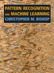
Bridges Bayesian statistics and machine learning, covering variational inference, Gaussian processes, and graphical models — the canonical advanced reference at this intersection.
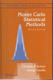
Provides rigorous mathematical coverage of MCMC and Monte Carlo methods that underpin all modern Bayesian computation, completing the theoretical picture.
Discussion
Keep reading
Paths that share books, cover the same subject, or open a related topic.