The Best Books to Learn Econometrics, In Order
This curriculum builds a rigorous, practical mastery of econometrics across four stages — starting from solid regression foundations, moving through causal inference and identification strategies, and culminating in advanced time-series and structural modeling. Because the learner starts at an intermediate level, early-stage hand-holding is skipped in favor of books that reward careful, engaged reading and build lasting intuition alongside technical depth.
Regression Foundations
IntermediateBuild a confident, rigorous understanding of OLS regression, its assumptions, diagnostics, and common violations — the bedrock vocabulary for everything that follows.
▸ Study plan for this stage
Pace: 8–10 weeks, ~40–50 pages/day (Stock first, then Greene; allow 1–2 weeks per major topic for integration and practice)
- The linear regression model: specification, parameters, and the interpretation of coefficients in levels and log-log forms
- Ordinary Least Squares (OLS) estimation: derivation, geometry, and why it minimizes the sum of squared residuals
- The Gauss-Markov assumptions and their role in guaranteeing BLUE (Best Linear Unbiased Estimator) properties
- Hypothesis testing and confidence intervals for regression coefficients using t-statistics and F-tests
- Heteroskedasticity: detection (visual inspection, Breusch-Pagan, White tests) and robust standard errors
- Autocorrelation: causes, detection (Durbin-Watson, correlogram), and implications for inference
- Multicollinearity: sources, detection (VIF, correlation matrices), and practical remedies
- Model specification and misspecification: omitted variables, functional form, and diagnostic residual analysis
- What are the five Gauss-Markov assumptions, and why does each one matter for the unbiasedness and efficiency of OLS?
- How do you interpret a regression coefficient when the dependent variable is in logs versus levels, and when both variables are in logs?
- What is heteroskedasticity, how do you detect it (name at least two tests), and how do robust standard errors address it?
- Explain the difference between autocorrelation and heteroskedasticity, and why autocorrelation violates the Gauss-Markov assumption of independent errors
- What is multicollinearity, how does it affect coefficient estimates and standard errors, and how would you diagnose it?
- How do you conduct an F-test for joint significance of multiple coefficients, and what does it tell you about model fit?
- Replicate a regression table from Stock (e.g., Chapter 4 or 5) using real data in R or Python; verify coefficient signs, magnitudes, and standard errors
- Generate synthetic data that violates one Gauss-Markov assumption (e.g., heteroskedastic errors), run OLS, and compare standard inference to robust standard errors
- Perform a Breusch-Pagan test and a White test for heteroskedasticity on a real dataset; interpret the test statistics and p-values
- Calculate the Variance Inflation Factor (VIF) for all regressors in a multi-variable regression; identify and discuss sources of multicollinearity
- Conduct residual diagnostics on a fitted OLS model: plot residuals vs. fitted values, create a Q-Q plot, and test for normality; identify any violations
- Estimate the same model in two functional forms (e.g., linear vs. log-log) and compare R², coefficients, and economic interpretation; discuss which is more appropriate
Next up: Mastery of OLS foundations—its assumptions, violations, and diagnostics—equips you to recognize when standard regression fails and prepares you for instrumental variables, panel data methods, and nonlinear models that relax or address these constraints.
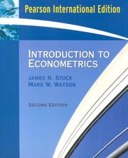
The gold-standard undergraduate-to-graduate bridge text. Its empirical-first approach ties every technique to real economic questions, giving the learner both intuition and formal grounding before moving to harder material.

The canonical graduate-level reference for classical econometrics. Read after Stock & Watson to formalize matrix-algebra notation, MLE, GLS, and panel methods that later causal-inference books assume as background.
Causal Inference & Identification
IntermediateUnderstand the potential-outcomes framework, the core identification strategies (IV, DiD, RD, matching), and how to think carefully about causality versus correlation in observational data.
▸ Study plan for this stage
Pace: 8–10 weeks, ~40–50 pages/day (mix of dense theory and applied examples)
- Potential outcomes framework (Rubin causal model): counterfactuals, treatment assignment, and the fundamental problem of causal inference
- Identification vs. estimation: what assumptions allow us to learn causal effects from observational data
- Instrumental variables (IV): using exogenous variation to isolate causal effects when treatment is endogenous
- Difference-in-differences (DiD): leveraging parallel trends and policy variation across groups/time to estimate treatment effects
- Regression discontinuity (RD): exploiting sharp cutoffs in treatment assignment to identify local causal effects
- Matching and propensity scores: balancing observable confounders to approximate randomization in observational settings
- The causal graph and directed acyclic graphs (DAGs): visualizing confounding, mediation, and selection bias
- Threats to identification: unobserved confounding, reverse causality, and measurement error in causal inference
- What is the potential outcomes framework, and why does it formalize the 'fundamental problem of causal inference'?
- Under what assumptions can instrumental variables identify a causal effect, and what does the LATE (Local Average Treatment Effect) represent?
- How does difference-in-differences estimation work, and what is the parallel trends assumption?
- What makes regression discontinuity a credible identification strategy, and when is it most convincing?
- How do matching and propensity score methods attempt to mimic randomization, and what limitations do they face?
- How can you use directed acyclic graphs (DAGs) to diagnose confounding and decide which variables to control for?
- Work through the potential outcomes notation in MHE Chapter 1 and Cunningham Chapter 1: write out the counterfactual outcomes and treatment effect for a concrete policy question (e.g., job training, education subsidy)
- Replicate an IV analysis from MHE (e.g., the Vietnam draft lottery or Angrist & Evans on fertility): download the data, estimate first and second stages, and interpret the LATE
- Implement a difference-in-differences estimator on a dataset with staggered treatment timing (e.g., state-level policy changes); compare results using standard DiD, event-study plots, and modern DiD estimators (e.g., Callaway & Sant'Anna)
- Design and execute a regression discontinuity analysis: identify a real cutoff (e.g., test score thresholds, age eligibility), visualize the discontinuity, and estimate the treatment effect with sensitivity checks
- Construct a propensity score model for a treatment of interest, perform matching or inverse-probability weighting, and assess covariate balance before and after
- Draw a DAG for a causal question you care about; identify confounders, mediators, and colliders; then explain which variables you would and would not control for in a regression
Next up: Mastering these core identification strategies equips you to critically evaluate causal claims in applied research and to design your own observational studies; the next stage will deepen your toolkit with advanced topics like sensitivity analysis, heterogeneous treatment effects, and machine learning methods for causal inference.

The definitive modern treatment of applied causal econometrics. Its conversational style and focus on the 'what's your identification strategy?' question reframes how economists think about regression, IV, DiD, and RD.

A highly accessible, code-rich companion that reinforces Angrist & Pischke's ideas with worked examples in Stata and R, making abstract identification strategies concrete and reproducible.
Bridges intuition and implementation with a strong focus on DAGs and research design thinking — read third to consolidate causal reasoning with a modern, graphical perspective.
Advanced Causal & Structural Methods
ExpertMaster treatment effects, program evaluation, structural econometrics, and the frontier methods used in academic and policy research.
▸ Study plan for this stage
Pace: 12–14 weeks, ~40–50 pages/day with 2–3 days/week for problem sets and coding
- Treatment effects and causal identification under unconfoundedness (propensity score methods, matching, regression adjustment)
- Difference-in-differences and event study designs for panel data
- Instrumental variables (IV) and two-stage least squares (2SLS) with weak instrument diagnostics
- Structural econometric models: static and dynamic discrete choice, and partial observability
- Nonlinear models for limited dependent variables (logit, probit, Tobit, count models) and their causal interpretation
- Program evaluation frameworks: randomized experiments, quasi-experiments, and sensitivity analysis
- Semiparametric and nonparametric methods (local polynomial regression, kernel estimation, series estimators)
- Machine learning and high-dimensional methods in econometrics for variable selection and prediction
- How do propensity score methods, matching, and regression adjustment each identify treatment effects, and when is each appropriate?
- What is the difference-in-differences estimator, what assumptions does it require, and how do you test for parallel trends?
- When is an instrument valid, how do you detect weak instruments, and what are the consequences of weak IV for inference?
- How do you specify and estimate a discrete choice model (logit/probit), and how do you recover treatment effects in nonlinear settings?
- What is the distinction between structural and reduced-form approaches, and when should you use each in program evaluation?
- How do semiparametric methods (e.g., local polynomial regression, series estimators) improve efficiency or robustness compared to parametric alternatives?
- Replicate a published difference-in-differences study using real panel data; test parallel trends assumption and report event-study plots
- Implement propensity score matching and inverse probability weighting (IPW) on a treatment assignment problem; compare estimates and assess covariate balance
- Conduct an IV analysis with weak instrument diagnostics (first-stage F-statistic, Anderson-Rubin test); document sensitivity to instrument strength
- Estimate a discrete choice model (logit or probit) on a binary or multinomial outcome; compute marginal effects and average treatment effects
- Build a dynamic panel model with lagged dependent variable; estimate via GMM (Arellano-Bond or Blundell-Bond) and interpret persistence
- Implement a semiparametric treatment effect estimator (e.g., Robinson's method or local polynomial regression) and compare to parametric alternatives
- Conduct a sensitivity analysis for unobserved confounding using bounds or calibration methods; document robustness of causal conclusions
- Use cross-validation and machine learning (e.g., LASSO, random forests) for variable selection in a high-dimensional treatment effect problem
Next up: This stage equips you with the full toolkit of modern causal inference and structural estimation, positioning you to either specialize in frontier topics (e.g., machine learning for causal inference, network econometrics, or dynamic structural models) or apply these methods to real-world policy and research problems with confidence in identification and robustness.
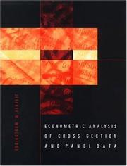
The authoritative graduate text on microeconometrics — covers GMM, panel data, count models, sample selection, and treatment effects with full rigor. Essential before tackling structural or frontier work.

A comprehensive companion to Wooldridge that goes deeper on simulation methods, duration models, and nonparametric approaches, rounding out the advanced practitioner's toolkit.
Time Series & Economic Data Modeling
ExpertDevelop fluency in time-series econometrics — stationarity, ARIMA, VAR, cointegration, and forecasting — essential for macroeconomics, finance, and any work with sequential economic data.
▸ Study plan for this stage
Pace: 12–14 weeks, ~40–50 pages/day (Hamilton: 8–9 weeks, ~45 pages/day; Tsay: 4–5 weeks, ~40 pages/day)
- Stationarity, unit roots, and the augmented Dickey-Fuller (ADF) test as foundational diagnostics for time-series data
- ARIMA(p,d,q) modeling: differencing, autoregressive and moving-average components, and model selection via ACF/PACF
- Vector autoregression (VAR) for multivariate systems, impulse-response analysis, and Granger causality
- Cointegration and error-correction models (VECM) for capturing long-run equilibrium relationships in economic data
- Volatility modeling: ARCH/GARCH frameworks for conditional heteroskedasticity in financial time series
- Forecasting evaluation: out-of-sample testing, forecast error metrics, and practical prediction strategies
- Structural breaks, regime shifts, and robustness checks in macroeconomic and financial applications
- Integration of Hamilton's theoretical foundations with Tsay's financial applications and computational methods
- What is stationarity, why does it matter for time-series regression, and how do you test for unit roots using the ADF test?
- How do you identify the order (p,d,q) of an ARIMA model using ACF and PACF plots, and what role does differencing play?
- Explain the difference between a VAR model and a system of simultaneous equations; when would you use each?
- What is cointegration, how does it relate to long-run equilibrium in economics, and how do you estimate a VECM?
- How do ARCH and GARCH models capture time-varying volatility, and why is this important for financial forecasting?
- Describe a complete forecasting workflow: model selection, estimation, out-of-sample evaluation, and interpretation of results.
- Replicate Hamilton's ADF test examples (Ch. 17) on real macroeconomic data (e.g., US GDP, inflation); interpret stationarity conclusions and compare results across lag specifications
- Fit ARIMA models to a univariate economic series (e.g., unemployment rate, stock price); use ACF/PACF to guide (p,d,q) selection, estimate the model, and validate residuals for white noise
- Build a VAR model for 3–4 related macroeconomic variables (e.g., output, inflation, interest rate); compute impulse-response functions and Granger causality tests; interpret economic implications
- Identify a cointegrated pair of financial or economic variables; estimate a VECM following Tsay's framework; analyze the error-correction term and long-run relationship
- Estimate GARCH(1,1) and ARCH models on daily stock returns; compare conditional volatility estimates, evaluate model fit, and discuss implications for risk management
- Conduct a full forecasting exercise: split data into training/test sets, fit competing models (ARIMA, VAR, VECM, GARCH as appropriate), generate out-of-sample forecasts, compute RMSE/MAE, and document which model performs best and why
Next up: Mastery of time-series econometrics equips you to handle dynamic economic relationships and volatility clustering, preparing you for advanced topics such as nonlinear models, high-dimensional VAR systems, and machine-learning approaches to forecasting in subsequent stages.

The definitive graduate-level reference for time-series econometrics. Its comprehensive coverage of ARMA, VAR, unit roots, and cointegration makes it the field's bible — read last because it demands the full econometric maturity built in prior stages.

Extends Hamilton's framework into financial applications — volatility modeling, GARCH, high-frequency data — providing a practical capstone for learners who work with market or macro-financial data.
Discussion
Keep reading
Paths that share books, cover the same subject, or open a related topic.