How to learn Machine learning
This curriculum takes you from zero machine learning knowledge to deep, practitioner-level mastery across four carefully sequenced stages. Each stage builds on the last — first developing intuition and math literacy, then hands-on coding skills, then rigorous theory, and finally the frontier of deep learning and research-grade understanding.
Foundations — Intuition & Big Picture
BeginnerUnderstand what machine learning is, why it matters, and how its core ideas work conceptually — without being overwhelmed by math or code.
▸ Study plan for this stage
Pace: 8–10 weeks total. Week 1–3: Read "The Hundred-Page Machine Learning Book" in full (~30–35 pages/day, ~3–4 sessions/week) — its brevity makes it ideal for building a clean mental map first. Week 4–10: Read Chapters 1–8 of "Hands-On Machine Learning with Scikit-Learn, Keras, and TensorFlow" (~20–25 pa
- What machine learning is and how it differs from classical rule-based programming (Burkov Ch. 1; Géron Ch. 1)
- The three learning paradigms: supervised, unsupervised, and reinforcement learning — with concrete real-world examples from both books
- The supervised learning setup: features, labels, training set, validation set, test set, and the prediction pipeline (Burkov Ch. 2–3; Géron Ch. 1–2)
- Bias–variance tradeoff and the twin dangers of underfitting vs. overfitting — why a model that memorizes training data fails in the real world (Burkov Ch. 4; Géron Ch. 4)
- Core algorithm families and their intuitions: linear/logistic regression, decision trees, k-NN, SVMs, and ensemble methods such as Random Forests and Gradient Boosting (Burkov Ch. 3–5; Géron Ch. 3–7)
- The end-to-end ML project workflow: problem framing → data collection → feature engineering → model selection → evaluation → deployment (Géron Ch. 2)
- Key evaluation metrics and why accuracy alone is misleading: precision, recall, F1-score, ROC-AUC, RMSE (Géron Ch. 3; Burkov Ch. 4)
- The role of data preprocessing and feature engineering — scaling, encoding, imputation — and why 'garbage in, garbage out' is the practitioner's first law (Géron Ch. 2 & 8; Burkov Ch. 5)
- In your own words, what is the difference between a machine learning system and a traditional software program? Use a concrete example from either book to illustrate.
- What distinguishes supervised, unsupervised, and reinforcement learning? For each paradigm, name one algorithm and one real-world use case discussed in the books.
- Why can a model with near-perfect training accuracy still fail badly on new data? Explain using the concepts of overfitting and the bias–variance tradeoff as introduced by Burkov.
- Walk through the end-to-end ML project checklist from Géron's Chapter 2. What happens at each stage, and what can go wrong if a stage is skipped?
- Why is accuracy often a poor metric for classification problems? What does Géron's Chapter 3 suggest using instead, and when would you prefer precision over recall (or vice versa)?
- What is feature engineering, and why do both Burkov and Géron treat it as one of the highest-leverage activities in any ML project?
- **Mental-model mapping (after Burkov):** Draw a one-page diagram of the ML landscape — place every algorithm family Burkov mentions on a 2-axis grid (supervised/unsupervised × parametric/non-parametric). Annotate each with one sentence of intuition. No code required.
- **End-to-end project walkthrough (Géron Ch. 2):** Follow Géron's California Housing notebook purely as a *reader*, not a coder — read every cell, predict what the output will be before running it, and write a one-paragraph plain-English summary of what each major block accomplishes.
- **Metric intuition exercise (Géron Ch. 3):** Invent two classification scenarios — one where false negatives are catastrophic (e.g., cancer screening) and one where false positives are costly (e.g., spam filtering). Write out which metric you'd optimize for each and why, citing the definitions from the book.
- **Bias–variance journal entry (Burkov Ch. 4):** Find a learning curve plot (Géron Ch. 4 provides one). Write a short paragraph diagnosing whether the model shown is underfitting, overfitting, or well-fit, and propose one concrete remedy for each case.
- **Algorithm family 'cheat cards':** For each of the five algorithm families covered (linear models, decision trees, k-NN, SVMs, ensembles), create a flashcard with: core intuition, one strength, one weakness, and the type of problem it suits best — drawn exclusively from Burkov and Géron's explanations.
- **Concept-to-real-world translation:** Choose any three algorithms from the books and find a news article or product (e.g., Netflix recommendations, email spam filters, medical diagnosis tools) that plausibly uses each. Write two sentences connecting the book's description of the algorithm to the real-world application.
Next up: By the end of this stage the reader holds a coherent conceptual map of the ML landscape and a feel for the full project lifecycle, which means the next stage — diving into the mathematics (linear algebra, calculus, probability) and systematic model training — will feel like filling in the *why* behind ideas already understood intuitively, rather than encountering them cold.

A concise, surprisingly complete survey of ML concepts written for beginners. Reading this first gives you a mental map of the entire field before diving into any single topic.
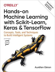
Bridges intuition and practice by pairing clear conceptual explanations with real Python code. Reading it here — before heavy theory — lets you build working models and develop concrete intuition simultaneously.
Mathematical Backbone
BeginnerDevelop the linear algebra, calculus, probability, and statistics literacy needed to read and derive ML algorithms from first principles.
▸ Study plan for this stage
Pace: 10–12 weeks total. Weeks 1–7: "Mathematics for Machine Learning" (~20–25 pages/day, focusing on Parts I & II — Linear Algebra, Analytic Geometry, Matrix Decompositions, Vector Calculus, and Probability & Distributions). Weeks 8–12: "An Introduction to Statistical Learning" (~15–20 pages/day, working
- Linear algebra fundamentals: vectors, matrices, dot products, norms, and linear transformations as covered in MML Chapters 2–4
- Matrix decompositions (LU, QR, eigendecomposition, SVD) and their geometric interpretations from MML Chapter 4
- Vector calculus: gradients, Jacobians, Hessians, and the chain rule as the engine behind backpropagation (MML Chapter 5)
- Probability theory: probability spaces, random variables, common distributions (Gaussian, Bernoulli, Binomial), expectation, and variance from MML Chapter 6
- Statistical inference: bias–variance tradeoff, maximum likelihood estimation, and Bayes' theorem as unified in MML Chapter 6 and revisited in ISL Chapter 2
- Model assessment: training vs. test error, cross-validation, and the concept of overfitting introduced in ISL Chapters 2 & 5
- Linear and logistic regression as the first concrete ML models, derived from the mathematical foundations built in MML (ISL Chapters 3 & 4)
- Regularization (Ridge and Lasso) as a bridge between optimization, probability (MAP estimation), and model selection (ISL Chapter 6)
- Given a matrix A, how do you compute its eigenvalues and eigenvectors, and what does the SVD of A reveal about the linear transformation it represents? (MML Ch. 4)
- How does the chain rule for vector-valued functions generalize to the Jacobian, and why is this the mathematical foundation of gradient-based learning? (MML Ch. 5)
- What is the relationship between maximizing a Gaussian likelihood and minimizing mean squared error in linear regression? Derive it from first principles. (MML Ch. 6, ISL Ch. 3)
- Explain the bias–variance tradeoff in your own words: what happens to each component as model complexity increases, and how does cross-validation help you find the sweet spot? (ISL Ch. 2 & 5)
- Why does adding an L2 penalty (Ridge) to the loss function correspond to placing a Gaussian prior on the model weights in a Bayesian framework? (ISL Ch. 6, MML Ch. 6)
- How does logistic regression use the sigmoid function and cross-entropy loss to turn a linear model into a probabilistic classifier? Derive the gradient of the loss. (ISL Ch. 4, MML Ch. 5–6)
- **MML Linear Algebra drills:** For each matrix decomposition covered (eigendecomposition, SVD), implement it from scratch in NumPy *without* calling `np.linalg.eig` or `np.linalg.svd`, then verify your result against the library function. Visualize how each decomposition transforms the unit circle.
- **Gradient derivation notebook:** Pick five scalar-valued functions from MML Chapter 5 exercises. Derive the gradient by hand, then verify numerically using finite differences: `(f(x+ε) − f(x−ε)) / 2ε`. This builds the muscle memory needed to derive ML loss gradients.
- **Probability simulation:** Using only NumPy's random module, simulate the Central Limit Theorem by drawing samples from three non-Gaussian distributions (uniform, exponential, Bernoulli). Plot the sampling distribution of the mean for n = 5, 30, 100 and connect the result to MML Chapter 6's discussion of Gaussians.
- **ISL Labs in Python:** Re-implement every R lab in ISL Chapters 3–6 using `scikit-learn` and `statsmodels`. For each model, print the coefficient estimates, compare them to the closed-form solution you derive by hand (e.g., β̂ = (XᵀX)⁻¹Xᵀy for OLS), and confirm they match.
- **Bias–variance experiment:** Using a synthetic polynomial dataset, train models of degree 1 through 10. Plot training error and 5-fold CV error on the same axes. Annotate the underfitting and overfitting regions and write a one-paragraph explanation linking the graph to ISL Chapter 2's theory.
- **Ridge vs. Lasso path:** Using the `Hitters` dataset from ISL Chapter 6, plot the full regularization path for both Ridge and Lasso as λ varies. Identify which coefficients shrink to exactly zero under Lasso and explain geometrically (using the ISL constraint-region diagrams) why Lasso produces sparsity while Ridge does not.
Next up: ">Mastering these mathematical and statistical foundations — gradients, probability, model fitting, and regularization — equips the reader to open any ML algorithm's "black box" and understand the optimization objectives, probabilistic assumptions, and generalization guarantees that will be explored in depth during the core ML algorithms stage.

Written specifically to fill the math gap for ML practitioners, covering linear algebra, calculus, and probability in a unified, application-focused way. Start here to build the language the rest of the curriculum is written in.

Introduces statistical thinking and classical ML models (regression, classification, resampling, trees) with gentle math and R examples. Solidifies the bridge between statistics and machine learning before moving to heavier texts.
Core Theory — Going Deeper
IntermediateMaster the theoretical underpinnings of classical machine learning algorithms, understand why they work, and learn to reason about generalization, bias-variance, and model selection rigorously.
▸ Study plan for this stage
Pace: 20–24 weeks total: ~14 weeks for Bishop's PRML (~3 chapters/week, ~35–45 pages/day, focusing on Chs. 1–4, 6–8, 9–10 deeply and skimming Chs. 11–14) + ~8–10 weeks for Hastie's ESL (~25–35 pages/day, prioritizing Chs. 2–5, 7–9, 15–16). Plan for 5 focused days/week, leaving 2 days for exercises and rev
- Probabilistic generative vs. discriminative models — Bishop Chs. 1–2, 4 ground every algorithm in a probability framework; understand likelihoods, priors, posteriors, and the role of Bayes' theorem in model inference
- Bias-variance tradeoff and the decomposition of generalization error — Bishop Ch. 3 (linear models) and ESL Ch. 2–3 introduce the formal decomposition; learn to diagnose underfitting vs. overfitting analytically, not just empirically
- Regularization as Bayesian prior — connect L2 (ridge) regularization to a Gaussian prior and L1 (lasso) to a Laplace prior via MAP estimation, covered in Bishop Ch. 3 and ESL Ch. 3
- Kernel methods and the kernel trick — Bishop Ch. 6 (Gaussian Processes) and ESL Ch. 5 (basis expansions) and Ch. 12 (SVMs) show how feature spaces can be implicitly infinite-dimensional; understand Mercer's theorem conceptually
- Expectation-Maximization (EM) algorithm — Bishop Ch. 9 derives EM rigorously for mixture models and beyond; understand the E-step/M-step as coordinate ascent on a lower bound of the log-likelihood
- Graphical models and conditional independence — Bishop Ch. 8 introduces directed (Bayesian networks) and undirected (Markov random fields) graphical models; learn d-separation and the message-passing algorithm
- Model selection and information criteria — ESL Ch. 7 covers AIC, BIC, cross-validation, and the bootstrap as principled tools for selecting model complexity; connect to the bias-variance tradeoff
- Ensemble methods and boosting theory — ESL Chs. 10 and 15–16 cover AdaBoost, gradient boosting, and random forests; understand why combining weak learners reduces variance and how forward stagewise additive modeling works
- Given a new dataset, how would you formally decompose its expected prediction error into bias², variance, and irreducible noise terms (as developed in ESL Ch. 2–3 and Bishop Ch. 3), and what model choices does that decomposition suggest?
- Explain why L2 regularization in linear regression is exactly equivalent to placing a zero-mean Gaussian prior on the weights and performing MAP estimation — walk through the math from Bishop Ch. 3.
- What is the EM algorithm doing geometrically? Describe the E-step and M-step in terms of a lower bound on the log-likelihood, and explain why convergence is guaranteed but not necessarily to a global optimum (Bishop Ch. 9).
- How does the kernel trick allow SVMs and Gaussian Processes to operate in potentially infinite-dimensional feature spaces without explicitly computing feature vectors, and what conditions must a kernel function satisfy (Bishop Ch. 6, ESL Ch. 12)?
- Compare AIC and BIC as model selection criteria: what loss function does each optimize, which penalizes complexity more heavily, and under what data-generating assumptions is each appropriate (ESL Ch. 7)?
- Why do ensemble methods like random forests and gradient boosting outperform single decision trees? Distinguish the variance-reduction mechanism of bagging from the bias-reduction mechanism of boosting using the theory in ESL Chs. 10 and 15.
- Derive ridge regression from scratch: start from the Gaussian likelihood + Gaussian prior, write out the MAP objective, differentiate, and arrive at the closed-form solution (w = (XᵀX + λI)⁻¹Xᵀy). Then implement it in NumPy and verify against scikit-learn's Ridge, sweeping λ and plotting the bias-variance curves — grounding Bishop Ch. 3 and ESL Ch. 3.
- Implement a Gaussian Mixture Model with the EM algorithm from scratch (no libraries): code the E-step (compute responsibilities) and M-step (update means, covariances, mixing coefficients), track the log-likelihood each iteration, and visualize cluster assignments on a 2D synthetic dataset. Compare convergence behavior with different random initializations (Bishop Ch. 9).
- Work through at least 3 end-of-chapter exercises from ESL Ch. 7 on model selection — specifically the ones requiring you to derive the optimism of training error and the in-sample prediction error. Write out every algebraic step by hand before checking.
- Build a kernel ridge regression implementation: choose an RBF kernel, construct the kernel matrix K, solve for dual coefficients, and make predictions. Experiment with the bandwidth parameter σ and regularization λ, plotting how each affects the fitted function on a 1D regression task. Relate your observations to the theory in Bishop Ch. 6.
- Implement AdaBoost from scratch using decision stumps as weak learners. Train it on a binary classification dataset, plot the training and test error as a function of the number of boosting rounds, and observe that test error often continues to fall even after training error reaches zero — then read ESL Ch. 10's margin-theory explanation for why this happens.
- Create a personal 'concept map' after finishing each book: draw nodes for every major algorithm covered (linear regression, logistic regression, SVM, GMM, random forest, etc.) and annotate each edge with the theoretical concept that connects them (e.g., 'both minimize a regularized loss', 'both are special cases of exponential family models'). Revise the map after ESL to integrate both books' pers
Next up: Mastering the probabilistic reasoning, generalization theory, and algorithmic foundations in Bishop and Hastie equips the reader with the mathematical vocabulary and intuition needed to tackle deep learning — where the same concepts of regularization, optimization landscapes, and model capacity reappear at vastly larger scale.
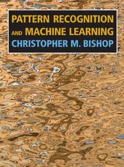
The definitive Bayesian treatment of machine learning. After the math stage, you now have the tools to work through its probabilistic models, graphical models, and inference methods — the gold standard for deep theoretical understanding.

Complements Bishop with a frequentist, statistics-first perspective on the same algorithms. Reading both back-to-back gives you a complete, dual-lens view of why ML models behave as they do.
Deep Learning — Modern Frontier
ExpertAchieve a research-grade understanding of deep neural networks — their architecture, optimization, theory, and state-of-the-art applications — and be equipped to read current ML papers.
▸ Study plan for this stage
Pace: 16–20 weeks total: Weeks 1–10 cover "Deep Learning" by Goodfellow (~25–30 pages/day, 6 days/week), focusing on Parts I–III sequentially; Weeks 11–20 cover "Dive into Deep Learning" by Zhang (~20–25 pages/day, 5 days/week), running every chapter's code interactively in parallel with reading.
- Feedforward networks, backpropagation, and the computational graph abstraction (Goodfellow Ch. 6–8)
- Regularization strategies: L1/L2, dropout, batch normalization, and early stopping (Goodfellow Ch. 7)
- Optimization algorithms: SGD, momentum, Adam, second-order methods, and loss-landscape geometry (Goodfellow Ch. 8)
- Convolutional Neural Networks: convolution as a structured linear operation, pooling, receptive fields, and modern architectures (AlexNet → ResNet) (Goodfellow Ch. 9; D2L Ch. 7–8)
- Recurrent Neural Networks, LSTMs, GRUs, and sequence-to-sequence modeling (Goodfellow Ch. 10; D2L Ch. 9–10)
- Attention mechanisms and the Transformer architecture: self-attention, multi-head attention, positional encoding (D2L Ch. 11)
- Generative models: VAEs and GANs — objectives, training dynamics, and mode collapse (Goodfellow Ch. 20; D2L Ch. 18)
- Deep learning theory: universal approximation, bias-variance in overparameterized regimes, and the role of depth vs. width (Goodfellow Ch. 5 & 6)
- Can you derive the full backpropagation update equations for a 3-layer MLP from first principles, including the chain rule through each activation function?
- What is the vanishing/exploding gradient problem, and how do architectural choices (residual connections, LSTMs, careful initialization) specifically address it?
- Compare and contrast at least four optimization algorithms covered in Goodfellow Ch. 8 — what problem does each solve, and under what conditions does one outperform another?
- How does the self-attention mechanism in the Transformer (D2L Ch. 11) differ fundamentally from the recurrent inductive bias of an LSTM, and what are the computational trade-offs?
- Explain the GAN training objective as a minimax game: what does convergence mean theoretically, why is it hard to achieve in practice, and what failure modes arise?
- How does batch normalization affect the loss landscape, and why does it interact with learning rate schedules in the way described in Dive into Deep Learning?
- Implement a full MLP with backpropagation from scratch using only NumPy (no frameworks), then verify gradients with finite differences — directly mirroring Goodfellow Ch. 6–8.
- Reproduce a ResNet-style residual block in PyTorch/MXNet using D2L Ch. 8 as a guide, then ablate the skip connections and plot training curves to observe the degradation problem firsthand.
- Train an LSTM and a Transformer encoder on the same sequence modeling task (e.g., character-level language model) using D2L Ch. 9–11 code notebooks; compare perplexity, training time, and attention visualizations.
- Implement and train a DCGAN on a small image dataset (e.g., Fashion-MNIST) following D2L Ch. 18; log discriminator/generator losses and experiment with at least two techniques to stabilize training (label smoothing, spectral normalization).
- Conduct a hyperparameter sweep (learning rate, batch size, dropout rate) on a CNN trained on CIFAR-10 using D2L's framework; write a one-page analysis connecting your empirical findings to the theoretical explanations in Goodfellow Ch. 7–8.
- Select one paper cited in either Goodfellow or D2L (e.g., the original Attention Is All You Need, or the Adam paper), read it in full, and write a two-page critical summary that maps each paper section back to the relevant book chapter.
Next up: Mastering the architectural foundations, optimization theory, and hands-on implementation skills in these two books equips the reader to engage directly with primary research literature, setting the stage for a research-methods or specialized-topics stage focused on reading and reproducing state-of-the-art ML papers across domains such as NLP, computer vision, or reinforcement learning.

The canonical textbook on deep learning, covering feedforward networks, CNNs, RNNs, optimization, and generative models with full mathematical rigor. The natural capstone after mastering classical ML theory.

Pairs deep theoretical content with runnable code in PyTorch and JAX, making it the perfect companion to Goodfellow for translating advanced concepts into modern implementations.
Discussion
Keep reading
Paths that share books, cover the same subject, or open a related topic.