How to learn Statistics
This curriculum takes you from everyday statistical intuition all the way to rigorous mathematical theory and modern applied practice. Each stage builds directly on the last — first developing conceptual fluency, then computational skill, then mathematical depth, and finally real-world mastery with modern tools.
Foundations: Building Statistical Intuition
BeginnerUnderstand what statistics is for, how data can mislead, and develop a confident intuitive grasp of core ideas like distributions, averages, variability, and probability — without heavy math.
▸ Study plan for this stage
Pace: 10–12 weeks total, roughly 20–25 pages/day. Week 1–2: "How to Lie with Statistics" (short, ~140 pages — read in one energetic burst, ~1 chapter/day). Weeks 3–7: "The Art of Statistics" (~400 pages — pace at 2–3 chapters/week, pausing to revisit examples). Weeks 8–12: "Naked Statistics" (~300 pages —
- Data can deceive: Huff's catalog of misleading graphs, truncated axes, biased samples, and ambiguous averages trains the eye to spot statistical manipulation before trusting any claim.
- The three averages (mean, median, mode) behave very differently and choosing the 'wrong' one — as Huff and Wheelan both illustrate — can radically distort a message.
- Distributions and variability: Spiegelhalter introduces the idea that a single summary number is almost never enough — spread, shape (skew, outliers), and the full distribution tell the real story.
- Probability as a language for uncertainty: Wheelan's intuitive treatment of probability, expected value, and the law of large numbers builds the mental scaffolding needed before any formal probability theory.
- Correlation vs. causation: all three books hammer this distinction — recognizing spurious correlations and confounding variables is a foundational critical-thinking skill.
- Sampling and bias: Huff's vivid examples (the WWII survivor-bias logic, biased polling) combined with Spiegelhalter's discussion of representative samples establish why how data is collected matters as much as the data itself.
- Statistical significance vs. practical significance: Spiegelhalter and Wheelan both warn that a result can be mathematically significant yet meaninglessly small in the real world.
- Communicating uncertainty honestly: Spiegelhalter's recurring theme — that good statistics is about quantifying and conveying what we don't know, not just what we do — reframes statistics as an ethical practice.
- After reading Huff, can you identify at least five specific techniques used to make statistics mislead, and find a real example of each in a news article or advertisement?
- How do mean, median, and mode differ, and in what real-world contexts (income distribution, home prices, test scores) would each be the most — or most deliberately misleading — choice?
- What is a distribution, and why does Spiegelhalter argue that showing the full distribution is almost always more informative than reporting a single average?
- What is the difference between correlation and causation, and how do confounding variables explain away seemingly compelling correlations (draw on examples from all three books)?
- What does Wheelan mean by 'expected value,' and how does it help evaluate everyday decisions involving risk and uncertainty?
- Why can a study with millions of participants produce a statistically significant result that is practically useless, and what questions should you ask to tell the difference?
- Lie-spotting log: While reading Huff, collect 10 real graphs or statistics from news sites, ads, or social media. Annotate each one identifying any of Huff's deceptive techniques (truncated axis, biased sample, missing denominator, etc.).
- Average showdown: Find a publicly available dataset (e.g., U.S. household income from the Census Bureau). Calculate the mean, median, and mode manually or in a spreadsheet. Write a one-paragraph 'spin' using each average to support a different narrative, then write a honest paragraph using all three.
- Distribution sketching: Pick any measurable phenomenon you encounter this week (your daily step count, coffee prices at a café, commute times). Record 20+ observations, plot a rough histogram by hand, and describe its shape: Is it symmetric? Skewed? Are there outliers? What does the shape tell you that the average alone wouldn't?
- Correlation hunt: Using a free tool like Google Dataset Search or Spurious Correlations (tylervigen.com), find three striking correlations. For each, brainstorm at least two plausible confounding variables or reasons the correlation is spurious — mirroring the reasoning Spiegelhalter and Wheelan model in their books.
- Probability journal: After finishing Wheelan's probability chapters, spend one week recording five daily decisions that involve uncertainty (weather, traffic, a purchase). For each, write an informal expected-value calculation and note whether your gut feeling matched the math.
- Rewrite the headline: Find five news headlines that make a statistical claim (e.g., 'X doubles your risk of Y'). Using concepts from all three books, rewrite each headline to be more accurate — adding base rates, confidence caveats, or sample-size context — and explain in one sentence what the original headline left out.
Next up: By finishing this stage, the reader has built a critical eye for data and a comfortable intuition for distributions, probability, and uncertainty — exactly the conceptual vocabulary needed to engage with the formal methods (hypothesis testing, regression, inference) that a more quantitative intermediate stage will introduce with rigor.

A short, witty classic that immediately trains the reader to think critically about data and statistical claims — the perfect first lens before learning the tools themselves.

A modern, concept-first tour of the entire statistical landscape by a leading statistician; builds genuine intuition for inference, uncertainty, and visualization before any formulas appear.
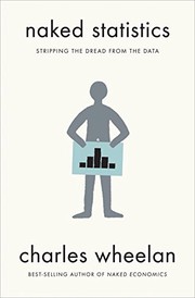
Covers probability, regression, and inference in plain English with vivid real-world examples, solidifying the vocabulary and mental models needed for the technical stages ahead.
Core Methods: Learning to Do Statistics
BeginnerMaster the standard toolkit — descriptive statistics, probability, hypothesis testing, confidence intervals, and simple regression — with enough worked examples to apply them independently.
▸ Study plan for this stage
Pace: 8–10 weeks, ~20–25 pages/day, 5 days/week — OpenIntro Statistics is ~430 pages; pace yourself with ~1 chapter per week, spending extra time on Chapters 4–6 (probability & inference) and revisiting worked examples before moving on
- Descriptive statistics: measures of center (mean, median, mode) and spread (variance, standard deviation, IQR), and how to choose between them
- Data visualization: histograms, box plots, scatterplots, and bar charts as tools for exploring distributions and relationships
- Probability foundations: sample spaces, the addition and multiplication rules, conditional probability, and independence
- Probability distributions: the normal distribution, Z-scores, and the binomial distribution as models for real-world randomness
- Sampling distributions and the Central Limit Theorem: why sample means behave predictably and how this underpins all inference
- Hypothesis testing: the logic of null vs. alternative hypotheses, p-values, significance levels (α), Type I/II errors, and one- and two-sample t-tests
- Confidence intervals: construction, correct interpretation ('95% of such intervals capture the true parameter'), and the relationship to hypothesis tests
- Simple linear regression: fitting a least-squares line, interpreting slope and intercept, R², residual analysis, and the conditions for inference
- Given a dataset, can you compute the mean, median, standard deviation, and IQR by hand and explain which summary is most appropriate when the data are skewed?
- What does the Central Limit Theorem guarantee, and why does it allow us to use the normal distribution even when the population is not normal?
- Walk through a complete hypothesis test (state hypotheses, check conditions, compute the test statistic and p-value, make a decision, write a conclusion in context) for a one-sample t-test.
- What is the correct interpretation of a 95% confidence interval, and what would happen to the interval width if you increased the sample size or raised the confidence level to 99%?
- In a simple linear regression output, what do the slope, intercept, and R² each tell you, and how do you check whether the conditions for regression inference are satisfied?
- What is the difference between a Type I and a Type II error, and how do the choices of α and sample size affect each?
- Work every end-of-chapter exercise in OpenIntro Statistics marked with a solution in the back — check your work immediately and write a one-sentence explanation of any mistake before moving on
- For each major dataset introduced in the book (e.g., county, email, loan data), reproduce the key summary statistics and plots by hand or in a free tool (R, Python, or even a spreadsheet), then compare to the book's figures
- Run 10 full hypothesis tests from scratch on real data you find (sports stats, weather records, public health data): state H₀ and Hₐ, verify conditions, compute t or Z, find the p-value, and write a plain-English conclusion
- Build a 95% and a 99% confidence interval for the same dataset, explain the difference in width, and then deliberately misstate the interpretation in three common wrong ways — then correct each one in writing
- Fit a simple linear regression to a dataset of your choice, plot the residuals vs. fitted values and a Q-Q plot of residuals, and write a paragraph assessing whether the four regression conditions (linearity, independence, constant variance, normality of residuals) are met
- Create a one-page 'cheat sheet' for each of the four inference procedures covered (one-sample t-test, two-sample t-test, proportion z-test, simple regression t-test) listing: conditions to check, formula, decision rule, and interpretation template
Next up: Mastering OpenIntro's core toolkit — especially the logic of inference and the mechanics of regression — gives you the procedural fluency and statistical intuition needed to tackle multiple regression, ANOVA, categorical data analysis, and model selection in a more advanced statistics course or textbook.

A free, rigorous, and highly readable textbook that reinforces hypothesis testing, regression, and ANOVA with real datasets, bridging the gap between concepts and computation.
Going Deeper: Probability & Mathematical Statistics
IntermediateUnderstand the mathematical foundations underlying statistical methods — probability theory, distributions, likelihood, and the formal logic of estimation and testing.
▸ Study plan for this stage
Pace: 12–16 weeks total: Weeks 1–6 cover Bertsekas's "Introduction to Probability" (~25–30 pages/day, focusing on chapters sequentially through combinatorics, discrete/continuous distributions, and limit theorems); Weeks 7–16 cover Wackerly's "Mathematical Statistics with Applications" (~20–25 pages/day,
- Sample spaces, events, and the axioms of probability (Bertsekas Ch. 1) — the rigorous set-theoretic foundation of all probability statements
- Conditional probability, independence, and Bayes' theorem (Bertsekas Ch. 1–2) — the engine behind inference and updating beliefs
- Discrete and continuous random variables: PMFs, PDFs, CDFs, and expectation/variance (Bertsekas Ch. 2–3)
- Key named distributions and their properties: Binomial, Poisson, Geometric, Exponential, Normal, Gamma, Beta (Bertsekas Ch. 2–3; Wackerly Ch. 3–4)
- Joint distributions, covariance, correlation, and transformations of random variables (Bertsekas Ch. 4; Wackerly Ch. 5–6)
- The Law of Large Numbers and the Central Limit Theorem — why sample means behave predictably (Bertsekas Ch. 5)
- Likelihood functions, sufficiency, and the principles of point estimation: MLE and method of moments (Wackerly Ch. 8–9)
- Confidence intervals and hypothesis testing: logic of Type I/II errors, p-values, power, and the Neyman–Pearson framework (Wackerly Ch. 8–10)
- Given a probability model, can you derive the conditional probability of an event and apply Bayes' theorem to update it with new information (as practiced in Bertsekas Ch. 1–2)?
- How do you compute the expectation and variance of a function of one or more random variables, and what do the results tell you about the distribution's shape and spread (Bertsekas Ch. 2–4)?
- Why does the Central Limit Theorem justify using the Normal distribution as an approximation in so many real-world settings, and what are its key assumptions and limitations (Bertsekas Ch. 5)?
- What is a likelihood function, and how does maximizing it yield a point estimator? How does the MLE compare to a method-of-moments estimator in terms of bias and efficiency (Wackerly Ch. 9)?
- How do you construct a confidence interval for a population mean or proportion, and what does the confidence level actually mean probabilistically (Wackerly Ch. 8)?
- What is the logical structure of a hypothesis test — null vs. alternative hypothesis, test statistic, rejection region, and the trade-off between Type I and Type II errors (Wackerly Ch. 10)?
- Work every odd-numbered problem in Bertsekas Ch. 1–2 on combinatorics and conditional probability; then re-derive Bayes' theorem from scratch without looking at the book to confirm you own the logic.
- For each named distribution covered (Binomial, Poisson, Exponential, Normal, Gamma), manually derive its mean and variance from the definition of expectation — do not just memorize formulas.
- Simulate the Law of Large Numbers and the CLT in Python or R: draw increasing sample sizes from a skewed distribution (e.g., Exponential) and plot how the sample-mean distribution converges to Normal; compare your plots to the theoretical predictions in Bertsekas Ch. 5.
- Using a small real dataset (e.g., from UCI ML Repository), hand-calculate the MLE for the parameter of a Poisson or Exponential model as developed in Wackerly Ch. 9, then verify with an optimizer in Python/R.
- Construct 90%, 95%, and 99% confidence intervals for a mean from the same dataset, then write a one-paragraph plain-English interpretation of each — explicitly avoiding the common misinterpretation that the parameter is 'probably in the interval.'
- Design and carry out a full hypothesis test (following Wackerly Ch. 10's framework) on a two-sample problem: state H₀ and H₁, choose α, compute the test statistic, find the p-value, state the conclusion, and calculate the power of the test against a specific alternative.
Next up: By internalizing probability theory (Bertsekas) and the formal machinery of estimation and testing (Wackerly), the reader has the mathematical vocabulary and logical scaffolding needed to critically engage with applied statistical modeling — regression, ANOVA, and beyond — in the next stage without treating formulas as black boxes.

Provides a rigorous yet accessible grounding in probability theory — the essential mathematical language for everything that follows in formal statistics.
A canonical intermediate textbook that derives the methods learned earlier from first principles, covering maximum likelihood, sufficient statistics, and asymptotic theory.
Modern Practice: Regression, Inference & Data Analysis
IntermediateApply statistical thinking to complex real-world data using regression modeling, model diagnostics, and causal reasoning — the skills used by working statisticians and data scientists.
▸ Study plan for this stage
Pace: 16–20 weeks total: ~10 weeks on "Regression and Other Stories" (~25–30 pages/day, focusing on Parts 1–4 deeply before moving on), then ~8–10 weeks on "The Elements of Statistical Learning" (~20–25 pages/day, with slower passes on dense chapters like 7, 10, and 12).
- Linear and logistic regression as generative models — understanding not just how to fit them but what assumptions they encode (Gelman, Parts 1–2)
- Predictive checking and model validation — using posterior predictive checks, residual plots, and cross-validation to diagnose model fit (Gelman, Chapters 11–12)
- Causal inference fundamentals — distinguishing predictive from causal models, understanding confounding, and the role of design (Gelman, Chapters 18–21)
- Bayesian workflow — iterative model building, prior selection, and the cycle of fit → check → revise (Gelman, throughout)
- Bias–variance tradeoff — the central tension in statistical learning that governs model complexity decisions (ESL, Chapter 2 & 7)
- Regularization methods — Ridge, Lasso, and elastic net as principled tools for controlling model complexity and handling high-dimensional data (ESL, Chapters 3–4)
- Tree-based and ensemble methods — decision trees, bagging, random forests, and boosting as flexible nonparametric learners (ESL, Chapters 9–10)
- Model selection and assessment — AIC, BIC, cross-validation, and the bootstrap as frameworks for choosing and evaluating models honestly (ESL, Chapter 7)
- After fitting a regression model in 'Regression and Other Stories,' what steps would you take to check whether the model's assumptions are reasonable, and what plots or statistics would you use?
- Gelman emphasizes the difference between a predictive and a causal interpretation of a regression coefficient — explain this distinction with a concrete example from the book.
- What is the bias–variance tradeoff as described in ESL, and why does minimizing training error alone lead to poor generalization?
- How do Ridge and Lasso regression differ in their shrinkage behavior, and under what data conditions would you prefer one over the other (ESL, Chapter 3)?
- Describe the mechanics of gradient boosting as presented in ESL Chapter 10 — what is being 'boosted,' and how does it relate to fitting residuals sequentially?
- How does cross-validation as a model-selection tool (ESL, Chapter 7) connect to the predictive-checking philosophy advocated throughout 'Regression and Other Stories'?
- **Regression workflow in R/Python (Gelman-style):** Take a real dataset (e.g., earnings, radon, or election data used in the book), fit a linear regression, simulate from the fitted model, and compare simulated vs. observed data distributions as a posterior predictive check.
- **Causal diagram exercise:** For any observational dataset of your choice, draw a DAG representing assumed causal structure, identify potential confounders, and re-run the regression from Gelman's framework with and without the confounder — document how coefficients change and what that implies.
- **Implement Ridge and Lasso from scratch (ESL Ch. 3):** Using only matrix operations in NumPy or R, implement the Ridge regression closed-form solution and compare coefficient paths against sklearn/glmnet as λ varies; plot the shrinkage paths.
- **Bias–variance decomposition experiment (ESL Ch. 2 & 7):** Simulate a dataset from a known polynomial function, fit models of increasing complexity (degree 1–10), and empirically estimate bias and variance across 200 bootstrap resamples — plot the classic U-shaped test error curve.
- **Random forest vs. boosting shootout (ESL Ch. 9–10):** On a real tabular dataset (e.g., UCI repository), tune and compare a random forest and a gradient boosted model (XGBoost or sklearn GradientBoosting) using proper k-fold CV; analyze feature importances and partial dependence plots.
- **Unified model-selection report:** Pick one dataset and one prediction task; apply at least four methods covered across both books (e.g., OLS, Lasso, random forest, boosting); use cross-validation to compare them on a held-out test set; write a one-page memo in the style of Gelman's case studies explaining your modeling choices, diagnostics, and conclusions.
Next up: Mastering regression diagnostics, regularization, and ensemble methods here builds the mathematical and practical fluency needed to tackle deeper probabilistic modeling, high-dimensional inference, or specialized domains (e.g., time series, causal ML, or Bayesian computation) in a more advanced stage.

The most practical and modern treatment of regression available; emphasizes model building, checking, and interpretation over mechanical computation, using compelling real examples.

Bridges classical statistics and machine learning, covering regularization, trees, and high-dimensional methods — essential for understanding how statistics scales to modern data.
Mastery: Bayesian Thinking & Statistical Theory
ExpertAchieve a deep, unified understanding of statistical inference through the Bayesian paradigm and advanced theory, enabling you to reason about any statistical problem from first principles.
▸ Study plan for this stage
Pace: 20–26 weeks total. Book 1 — "Bayesian Data Analysis" (Gelman): ~14–16 weeks, reading roughly 20–25 pages/day, 5 days/week, with one full review day per week. Book 2 — "Statistical Inference" (Casella): ~6–10 weeks, reading roughly 20–25 pages/day, 5 days/week, revisiting Gelman chapters alongside Ca
- Bayes' theorem as a complete inference engine: prior, likelihood, and posterior construction (Gelman, Ch. 1–3)
- Prior specification: conjugate priors, weakly informative priors, and prior predictive checks (Gelman, Ch. 2–5)
- Posterior summarization: point estimates, credible intervals, and posterior predictive distributions (Gelman, Ch. 2–4)
- Hierarchical (multilevel) models and partial pooling as a principled solution to the bias-variance tradeoff (Gelman, Ch. 5–6)
- Markov Chain Monte Carlo (MCMC): Metropolis-Hastings, Gibbs sampling, Hamiltonian Monte Carlo, and convergence diagnostics (Gelman, Ch. 11–12)
- Bayesian model checking, comparison, and selection: posterior predictive checks, LOO-CV, WAIC, and Bayes factors (Gelman, Ch. 6–7)
- Likelihood theory and sufficiency: sufficient statistics, the factorization theorem, exponential families, and the likelihood principle (Casella, Ch. 3–6)
- Decision theory and optimality: risk functions, admissibility, minimaxity, and the connection between Bayes estimators and frequentist optimality (Casella, Ch. 7–8)
- Given a new data-generating problem, how do you construct a full Bayesian model — choosing a likelihood, specifying a prior, and deriving or approximating the posterior — as outlined in Gelman's workflow?
- What is the difference between a posterior predictive check and a prior predictive check, and how does each serve model criticism in Gelman's framework?
- How do hierarchical models in Gelman achieve partial pooling, and why is this preferable to either complete pooling or no pooling in grouped data settings?
- How do you diagnose MCMC convergence using R-hat, effective sample size, and trace plots as described in Gelman, and what do failures in each diagnostic imply about your sampler?
- From Casella's treatment, what does it mean for a statistic to be sufficient, and how does the Rao-Blackwell theorem connect sufficiency to the improvement of estimators?
- How does Casella's decision-theoretic framework unify Bayesian and frequentist estimation, and under what conditions is a Bayes estimator also minimax or admissible?
- Gelman workflow drill: For at least three datasets of your choice (e.g., count data, continuous outcomes, binary outcomes), write out the full Bayesian model specification — likelihood, prior, posterior derivation — by hand before touching any software, then implement in Stan or PyMC and compare your analytic result to the sampled posterior.
- Prior sensitivity analysis: For one of your models, systematically vary the prior (from very diffuse to strongly informative) and plot how the posterior and posterior predictive distribution shift; write a one-page interpretation of what this reveals about the data's informativeness, as Gelman's workflow demands.
- Hierarchical model implementation: Replicate the 8-schools example from Gelman Ch. 5 from scratch — code the no-pooling, complete-pooling, and partial-pooling models, compare their estimates and uncertainty, and explain in writing why partial pooling is the principled choice.
- MCMC diagnostics lab: Deliberately mis-specify a sampler (e.g., too few warmup steps, poor initialization) on a model from Gelman, then systematically apply all convergence diagnostics (R-hat > 1.01, low ESS, trace plot inspection, pairs plots) to identify and fix each failure mode.
- Sufficiency and Rao-Blackwell exercise (Casella): For the Poisson and Normal families, identify a complete sufficient statistic, construct an unbiased estimator, apply the Rao-Blackwell theorem to improve it, and verify the result achieves the Cramér-Rao lower bound where applicable.
- Decision theory synthesis: Pick one estimation problem (e.g., estimating a normal mean) and analyze it under both Casella's frequentist decision-theoretic framework (risk, admissibility, minimaxity) and Gelman's Bayesian framework (posterior loss minimization); write a two-page essay reconciling the two perspectives and identifying where they agree and diverge.
Next up: Mastering Bayesian inference through Gelman's applied workflow and Casella's rigorous theoretical foundations equips the reader to engage with specialized or research-level literature — such as nonparametric Bayes, causal inference, or machine learning theory — where first-principles statistical reasoning is the entry requirement.
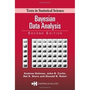
The definitive graduate-level text on Bayesian statistics; reading it after the previous stages lets you see the full inferential framework and compare it critically with frequentist methods.
A rigorous, comprehensive treatment of classical inference theory — sufficiency, completeness, UMVUEs, and decision theory — that ties together everything learned across the curriculum.
Discussion
Keep reading
Paths that share books, cover the same subject, or open a related topic.