The Best Books to Learn Causal Inference, In Order
This curriculum builds a rigorous, end-to-end mastery of causal inference — from intuitive graphical reasoning through counterfactual theory to cutting-edge econometric and machine-learning methods. Because the starting level is intermediate, the path skips purely introductory statistics and instead opens with accessible but substantive treatments, then steadily advances toward technical depth in potential outcomes, structural causal models, and modern identification strategies.
Causal Intuition & Graphical Foundations
IntermediateBuild a solid mental model of causation vs. correlation, learn to draw and read causal diagrams (DAGs), and understand confounding, colliders, and d-separation without heavy math.
▸ Study plan for this stage
Pace: 8–10 weeks, ~25–30 pages/day (mix of reading and diagram practice)
- Causation vs. correlation: why statistical association alone cannot establish causal claims
- Causal diagrams (DAGs): nodes as variables, arrows as direct causal relationships, and how to construct them from domain knowledge
- Confounding: how unmeasured or uncontrolled common causes bias causal estimates
- Colliders and selection bias: why conditioning on certain variables can create spurious associations
- d-separation and conditional independence: graphical rules for determining which variables must be controlled to identify causal effects
- The three rungs of the causal ladder: association, intervention, and counterfactuals
- Backdoor and frontdoor criteria: practical rules for identifying causal effects from observational data
- Causal identification: determining when a causal effect can be estimated from data given a causal diagram
- What is the fundamental difference between correlation and causation, and why can't randomized controlled trials always be conducted?
- How do you construct a causal DAG from domain knowledge, and what does an arrow between two variables represent?
- What is a confounder, and how does it bias causal estimates? Can you identify confounders in a given DAG?
- What is a collider, and why does conditioning on a collider create spurious association between its parents?
- What is d-separation, and how do you use it to determine which variables must be controlled to estimate a causal effect?
- Given a causal diagram, can you apply the backdoor criterion to determine whether a causal effect is identifiable from observational data?
- Draw causal DAGs for 5–6 real-world scenarios (e.g., smoking → lung cancer, education → income, social media use → mental health) and label confounders, mediators, and colliders
- For each DAG, identify all backdoor paths and determine which variables must be controlled using the backdoor criterion
- Practice d-separation: given a DAG and a pair of variables, determine whether they are d-separated conditional on a given set of variables
- Analyze 3–4 case studies from Pearl's books (e.g., the Berkeley admissions paradox, Monty Hall problem) and explain the role of colliders and selection bias
- Construct a causal diagram for a dataset you're familiar with (e.g., from your field), identify confounders, and propose a control strategy
- Work through Pearl's causal ladder exercises: for a given causal question, determine which rung (association, intervention, counterfactual) is needed and why
Next up: This stage equips you with the graphical language and intuition to represent causal structures and identify when effects are estimable—the foundation for the next stage, where you'll learn the statistical and algorithmic methods to actually estimate those effects from data.

Pearl's accessible manifesto introduces the Ladder of Causation — association, intervention, counterfactuals — and DAG-based reasoning in plain language. Reading this first gives you the conceptual vocabulary every later book assumes.

This short, rigorous companion translates the intuitions from The Book of Why into formal do-calculus, adjustment formulas, and identification — the essential bridge before tackling potential-outcomes literature.
Potential Outcomes & Applied Identification
IntermediateMaster the Rubin potential-outcomes framework, understand the core identification strategies (RCTs, IV, DiD, RD), and be able to critically evaluate observational study designs.
▸ Study plan for this stage
Pace: 8–10 weeks, ~40–50 pages/day (mix of dense theory and worked examples)
- The Rubin potential-outcomes framework: counterfactuals, treatment assignment, and the fundamental problem of causal inference
- The role of randomization in RCTs and why it solves the selection problem
- Instrumental variables (IV): using exogenous variation to identify causal effects when treatment is endogenous
- Difference-in-differences (DiD): exploiting parallel trends and policy variation across groups/time to isolate treatment effects
- Regression discontinuity (RD): leveraging sharp cutoffs in treatment assignment to estimate local causal effects
- Selection bias, omitted variable bias, and how each identification strategy addresses these threats
- Internal vs. external validity: when and why causal estimates generalize beyond the study population
- Critical evaluation of observational studies: assessing credibility of assumptions (exclusion restrictions, parallel trends, continuity)
- What is the fundamental problem of causal inference, and how does the potential-outcomes framework formalize it?
- Why does randomization solve the selection problem, and what assumptions must hold for an RCT to yield valid causal estimates?
- What is an instrumental variable, what is the exclusion restriction, and why is it crucial for IV identification?
- Explain the parallel trends assumption in difference-in-differences and describe a realistic scenario where it might fail.
- What is a regression discontinuity design, and why does a sharp cutoff in treatment assignment enable causal identification?
- How would you critically evaluate an observational study design to assess whether its causal claims are credible?
- Work through Angrist's RCT examples (e.g., the NSW job training study) and replicate the calculations to understand how randomization eliminates selection bias.
- Implement an IV estimator (2SLS) on a dataset with endogenous treatment; verify the first-stage F-statistic and discuss weak instrument concerns.
- Construct a difference-in-differences estimate using real or simulated data with treatment variation across groups and time; check the parallel trends assumption visually and formally.
- Design and execute a regression discontinuity analysis on a dataset with a known cutoff (e.g., education policy, age-based eligibility); examine robustness to bandwidth choice.
- Critically appraise a published observational study from your field: identify the identification strategy, list the key assumptions, and assess whether they are plausible.
- Write a short memo (1–2 pages) comparing the internal and external validity of an RCT vs. an IV or DiD study on the same topic; discuss trade-offs.
Next up: This stage equips you with the conceptual and practical toolkit to identify causal effects in diverse settings; the next stage will deepen your ability to handle violations of these core assumptions, combine multiple strategies, and tackle modern challenges like heterogeneous treatment effects and causal machine learning.

The canonical applied econometrics text that teaches regression, IV, DiD, and RD through real empirical examples. Its irreverent style makes demanding material approachable and sets the standard vocabulary for the applied causal inference community.

A freely available, example-rich complement to Angrist that walks through each identification strategy with code (Stata/R). Reading it after Mostly Harmless reinforces and extends the same ideas with more worked examples and modern methods like synthetic control.
Rigorous Counterfactual Theory
ExpertDevelop a deep, unified theoretical understanding of causality by connecting potential outcomes, structural causal models, and the formal conditions for identification and inference.
▸ Study plan for this stage
Pace: 12–14 weeks, ~40–50 pages/day (Pearl: 8 weeks; Imbens & Wooldridge: 4–6 weeks). Allocate 2–3 days per major chapter for deep engagement with proofs and examples.
- Potential outcomes framework (Rubin causal model): definition of treatment effects, SUTVA, and the fundamental problem of causal inference
- Structural Causal Models (SCMs): graphical representation, causal mechanisms, and the do-calculus for interventional reasoning
- Identification: conditions for moving from observational data to causal parameters (backdoor, frontdoor, instrumental variables)
- Confounding, mediation, and collider bias: how causal graphs reveal which variables to control for and which to avoid
- Causal discovery and constraint-based methods: learning causal structure from data and assumptions
- Unconfoundedness and ignorability: formal assumptions underlying causal inference in observational studies
- Sensitivity analysis: quantifying robustness to hidden bias and unmeasured confounding
- Estimation and inference: translating identification results into estimators (matching, regression, doubly robust methods)
- What is the fundamental problem of causal inference, and how do potential outcomes and SCMs each address it?
- Explain the do-calculus and how it enables causal reasoning from observational distributions. What are the three rules?
- What conditions must hold for the backdoor criterion to justify controlling for a set of covariates? Provide a concrete example.
- How do the frontdoor criterion and instrumental variables identify causal effects when backdoor adjustment is not possible?
- What is SUTVA, why is it critical, and under what real-world scenarios might it be violated?
- Describe the relationship between a causal graph, the Markov condition, and the set of conditional independencies implied by the graph.
- What is unconfoundedness (conditional ignorability), and how does it differ from randomization? What can and cannot be tested from data alone?
- How would you design and interpret a sensitivity analysis to assess robustness to hidden confounding in an observational study?
- Pearl's *Causality* (Ch. 1–3): Draw causal graphs for 3–4 real-world scenarios (e.g., smoking→lung cancer, education→earnings); identify confounders, mediators, and colliders; apply the backdoor criterion to determine valid adjustment sets.
- Pearl's *Causality* (Ch. 4): Manually apply the three rules of do-calculus to derive causal effects in 2–3 non-trivial causal graphs; verify your results using Pearl's graphical criteria (backdoor, frontdoor).
- Imbens & Wooldridge (Ch. 1–2): Translate 2–3 research questions into potential outcomes notation; define treatment effects (ATE, CATE, ITT); identify which are identified under different assumptions.
- Imbens & Wooldridge (Ch. 3–4): For a real dataset (or simulated data), implement matching, regression adjustment, and doubly robust estimation; compare results and discuss sensitivity to unconfoundedness.
- Causal graph learning: Use constraint-based methods (e.g., PC algorithm concepts from Pearl) to infer causal structure from simulated data with known ground truth; evaluate accuracy.
- Sensitivity analysis exercise: Take an observational study result and compute bounds on the causal effect under varying degrees of hidden confounding (using Imbens's sensitivity framework); interpret the robustness of conclusions.
Next up: This stage establishes the theoretical foundations—potential outcomes, SCMs, identification, and unconfoundedness—that are essential for the next stage, which will likely focus on practical applications, advanced estimation techniques (e.g., machine learning for causal inference, heterogeneous treatment effects), and real-world case studies where these principles are deployed to answer substantive
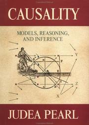
Pearl's magnum opus provides the full mathematical treatment of DAGs, do-calculus, counterfactuals, and identifiability. After the Primer and applied econometrics work, readers are ready to absorb its depth and see how both frameworks unify.

Imbens and Rubin's authoritative textbook gives the most thorough formal treatment of the potential-outcomes framework, covering assignment mechanisms, matching, IV, and sensitivity analysis — essential for anyone who wants to do or referee serious empirical work.
Modern Methods & Machine Learning for Causal Inference
ExpertIntegrate causal reasoning with high-dimensional data and machine learning tools — including double/debiased ML, causal forests, and policy evaluation — to handle real-world complexity.
▸ Study plan for this stage
Pace: 8–10 weeks, ~40–50 pages/day with 2–3 days per week for exercises and review
- Causal models as directed acyclic graphs (DAGs) and their connection to observational and interventional distributions
- Identifiability: when causal effects can be recovered from observational data (backdoor, frontdoor, instrumental variables)
- Markov and faithfulness assumptions: their role in causal discovery and limitations
- Causal discovery algorithms (PC, FCI, GES) and their assumptions, output interpretation, and practical constraints
- Handling hidden confounders and selection bias: methods for sensitivity analysis and bounds on causal effects
- Integration of machine learning with causal inference: avoiding pitfalls of naive prediction in causal settings
- Causal reasoning under high-dimensional data: variable selection, regularization, and double/debiased machine learning foundations
- Policy evaluation and heterogeneous treatment effects: moving from average effects to individualized decision-making
- What is the difference between observational and interventional distributions, and how do causal models formalize this distinction?
- Under what conditions can causal effects be identified from observational data? Explain the backdoor criterion and at least one alternative identification strategy.
- What are the Markov and faithfulness assumptions, why are they important for causal discovery, and what happens when they are violated?
- How do causal discovery algorithms (e.g., PC, FCI) work, what assumptions do they require, and what are the practical limitations of their output?
- Why is naive machine learning prediction problematic in causal settings, and how does the causal inference perspective change feature selection and model building?
- How can you assess robustness of causal conclusions when hidden confounders may exist? What do sensitivity analyses and bounds tell you?
- Construct DAGs for 3–4 real-world scenarios (e.g., education → earnings, smoking → disease, marketing → sales); identify confounders, mediators, and colliders; verify d-separation by hand.
- Apply the backdoor criterion to identify minimal adjustment sets in your DAGs; compare with frontdoor and instrumental variable approaches where applicable.
- Implement or walk through the PC algorithm on a small synthetic dataset (10–15 variables); document assumptions, output, and how the skeleton and orientation rules work.
- Simulate observational data from a known causal model; run a causal discovery algorithm (e.g., using the causalml or DoWhy Python packages); compare recovered graph to ground truth and analyze false positives/negatives.
- Conduct a sensitivity analysis on a causal estimate: assume an unmeasured confounder with varying strength and direction; compute bounds on the true causal effect.
- Take a published observational study; critically evaluate its causal assumptions (Markov, faithfulness, no hidden confounders); propose what additional data or methods would strengthen causal claims.
Next up: This stage establishes the theoretical and algorithmic foundations for causal reasoning with complex data, preparing you to apply double/debiased machine learning, causal forests, and policy evaluation methods that leverage these principles to estimate heterogeneous effects and optimize interventions in high-dimensional settings.

Peters, Janzing, and Schölkopf connect causal structure learning, invariant prediction, and machine learning in a mathematically precise way, representing the frontier where causal inference meets modern AI research.
Discussion
Keep reading
Paths that share books, cover the same subject, or open a related topic.