The Best Books to Learn Digital Signal Processing, In Order
Since the learner starts at an expert level, this curriculum skips elementary introductions and moves immediately into rigorous, mathematically mature DSP theory — covering discrete-time systems, filter design, spectral analysis, and advanced topics like multirate processing and statistical signal processing. Each stage sharpens a distinct layer of mastery, from solid theoretical grounding through research-grade depth.
Rigorous Foundations
BeginnerEstablish a mathematically precise framework for discrete-time signals and systems, the Z-transform, DFT, and classic filter design — the shared vocabulary for everything that follows.
▸ Study plan for this stage
Pace: 8–10 weeks, ~40–50 pages/day (Oppenheim: weeks 1–6; Lyons: weeks 7–10)
- Discrete-time signals and sequences: representation, classification (periodic, aperiodic, energy/power), and the impulse and step sequences as fundamental building blocks
- Linear time-invariant (LTI) systems: convolution as the core operation, impulse response characterization, and causality/stability conditions
- Z-transform: definition, region of convergence (ROC), inverse transforms, and solving difference equations—the bridge between time and frequency domains
- Discrete Fourier Transform (DFT): derivation from the Z-transform, periodicity, circular convolution, and the Fast Fourier Transform (FFT) algorithm
- Frequency response and filtering: magnitude and phase response, ideal vs. practical filters, and the relationship between poles/zeros and filter behavior
- Classic filter design methods: FIR and IIR design techniques (windowing, bilinear transform), filter specifications, and trade-offs between filter types
- Sampling theorem and reconstruction: Nyquist criterion, aliasing, and the connection between continuous and discrete-time signals
- Practical DSP implementation: finite precision effects, computational complexity, and real-world constraints in filter realization
- What is the Z-transform, how do you compute it, and why is the region of convergence (ROC) critical for uniqueness and causality?
- How does convolution relate to LTI systems, and how do you use it to compute the output of a discrete-time system given an input and impulse response?
- What is the Discrete Fourier Transform, how does it relate to the Z-transform, and what is circular convolution?
- How do you design an FIR filter using windowing, and what are the trade-offs between window types in terms of transition width and stopband ripple?
- What is the bilinear transform, how do you use it to convert an analog filter design to a digital filter, and what are its limitations?
- What does the sampling theorem tell you about the relationship between continuous and discrete signals, and what is aliasing?
- Compute the Z-transform and ROC for 5–6 sequences of varying complexity (exponential, polynomial, finite-length); verify causality and stability from pole locations
- Perform hand convolution for 3–4 pairs of sequences (finite and infinite length); verify results using the Z-transform and frequency domain methods
- Compute the DFT by hand for 2–3 short sequences (N ≤ 8); then implement FFT in Python/MATLAB and verify against direct DFT for larger sequences
- Design an FIR lowpass filter using rectangular, Hamming, and Blackman windows; compare magnitude responses, transition widths, and stopband attenuation
- Design an IIR Butterworth filter using the bilinear transform: specify passband/stopband frequencies and ripple, compute analog prototype, then digitize and implement
- Simulate aliasing by sampling a continuous sinusoid above and below the Nyquist frequency; visualize the effect in both time and frequency domains
Next up: This stage equips you with the mathematical vocabulary and core algorithms (Z-transform, DFT, filter design) needed to tackle advanced topics like multirate processing, adaptive filtering, and spectral estimation in the next stage.

The canonical graduate-level DSP textbook. Its rigorous treatment of the Z-transform, DTFT, DFT, and FIR/IIR filter design sets the gold standard and is the reference every subsequent book assumes you know.
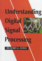
Read immediately after Oppenheim to solidify intuition: Lyons excels at geometric and visual explanations of concepts (especially the DFT and complex baseband) that Oppenheim states formally, bridging theory and practice.
Fourier Analysis & Spectral Estimation
IntermediateDevelop deep mastery of the Fourier transform in all its forms, windowing, leakage, and modern spectral estimation methods used in research and engineering.
▸ Study plan for this stage
Pace: 8–10 weeks, ~40–50 pages/day (Bracewell: 4–5 weeks; Percival: 4–5 weeks). Allocate 2–3 days per major topic for integration and hands-on work.
- Fourier transform fundamentals: definition, properties (linearity, scaling, shifting, convolution), and the relationship between time and frequency domains
- Discrete Fourier Transform (DFT) and Fast Fourier Transform (FFT): computational efficiency, aliasing, and the Nyquist criterion
- Windowing functions and spectral leakage: how window choice (Hann, Hamming, Blackman) affects frequency resolution and sidelobe behavior
- Power spectral density (PSD) estimation: periodogram, Welch's method, and bias-variance tradeoffs in spectral estimation
- Parametric spectral estimation methods: autoregressive (AR) models, maximum entropy method (MEM), and model order selection
- Practical spectral analysis: preprocessing, detrending, zero-padding, and interpretation of real-world signals
- Leakage, picket-fence effect, and scalloping loss: physical understanding and mitigation strategies
- Multitaper methods and modern estimation techniques for improved spectral resolution and reduced variance
- Explain the Fourier transform's core properties (linearity, convolution theorem, Parseval's theorem) and derive how they apply to a simple signal like a rectangular pulse.
- What is spectral leakage, why does it occur, and how do different window functions (Hann, Hamming, Blackman) trade off main-lobe width against sidelobe attenuation?
- Compare the periodogram, Welch's method, and multitaper methods: what are their bias and variance characteristics, and when should you use each in practice?
- Describe the relationship between signal length, frequency resolution, and the Nyquist frequency. How does zero-padding affect the DFT without improving true resolution?
- What is the picket-fence effect and scalloping loss? How do they manifest in spectral estimates and what practical steps mitigate them?
- Explain autoregressive (AR) spectral estimation: how does it differ from nonparametric methods, and how do you select the model order?
- Compute the Fourier transform analytically for 3–4 simple signals (e.g., rectangular pulse, Gaussian, sinusoid) using Bracewell's tables and properties; verify numerically with FFT.
- Implement the DFT and FFT algorithms from scratch (or study existing implementations); measure computational time scaling and verify correctness against NumPy/SciPy.
- Generate a synthetic signal with known frequency components; apply 4–5 different windows (rectangular, Hann, Hamming, Blackman, Kaiser) and plot the resulting spectrograms to visualize leakage and resolution tradeoffs.
- Estimate the power spectral density of a real signal (e.g., audio, seismic, or sensor data) using periodogram, Welch's method, and multitaper methods; compare bias, variance, and interpretability.
- Demonstrate the picket-fence effect and scalloping loss by estimating a sinusoid at frequencies that fall between DFT bins; show how windowing and zero-padding affect the estimate.
- Fit an autoregressive (AR) model to a time series using Yule-Walker or Burg's method; estimate the spectral density from the AR coefficients and compare to nonparametric methods.
Next up: Mastery of Fourier analysis and spectral estimation provides the mathematical and practical foundation for advanced topics such as time-frequency analysis (wavelets, spectrograms), adaptive filtering, and signal detection in noise—all of which rely on understanding how signals decompose in the frequency domain and how to estimate their spectral content accurately.
A uniquely intuitive yet thorough treatment of Fourier theory across continuous and discrete domains; its graphical approach and breadth of applications build the kind of Fourier fluency that purely algebraic texts miss.
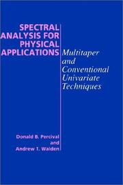
The definitive modern reference on spectral estimation — multitaper methods, bias-variance tradeoffs, and confidence intervals — essential for anyone doing serious frequency-domain analysis of real data.
Filter Design & Multirate Systems
IntermediateMaster advanced filter design techniques, polyphase structures, multirate signal processing, and filter banks — the engine behind audio codecs, SDR, and modern communications.
▸ Study plan for this stage
Pace: 8–10 weeks, ~40–50 pages/day (Vaidyanathan: 4–5 weeks; Porat: 3–4 weeks, with 1–2 weeks for integration and projects)
- Polyphase decomposition and noble identities for efficient filter implementation
- Multirate signal processing: decimation, interpolation, and rate conversion with minimal aliasing
- Filter bank theory: perfect reconstruction (PR) conditions and orthogonal/biorthogonal filter banks
- Subband decomposition and energy compaction for compression applications
- Design of FIR and IIR filters for multirate systems using frequency masking and spectral shaping
- Lattice structures and cascade realizations for numerical stability and modularity
- Wavelet filter banks and their connection to multiresolution analysis
- Practical implementation trade-offs: computational cost, memory, and real-time constraints
- What are the noble identities and how do they enable efficient polyphase filter implementations?
- Derive the perfect reconstruction conditions for a two-channel filter bank and explain how to verify them.
- How do decimation and interpolation relate to aliasing, and what role does the anti-aliasing filter play?
- Compare the computational complexity of direct convolution versus polyphase filtering for a decimation-by-M system.
- What is the relationship between filter bank design and wavelet decomposition, and why is energy compaction important for compression?
- Given a multirate system specification (sample rates, passband ripple, stopband attenuation), design an appropriate filter and justify your choice of structure (direct, polyphase, lattice).
- Implement polyphase decomposition of a given FIR filter and verify the noble identities numerically using MATLAB/Python.
- Design a two-channel perfect reconstruction filter bank (using Vaidyanathan's methods) and test PR on synthetic signals; measure reconstruction error.
- Build a multirate decimator (M=4) with anti-aliasing filter; compare output with and without proper filtering to observe aliasing artifacts.
- Implement a cascade of interpolation and decimation stages (rate conversion, e.g., 44.1 kHz → 48 kHz) and measure computational savings using polyphase structures.
- Design a wavelet filter bank (e.g., Daubechies-like) following Porat's treatment; apply to a test signal and visualize subband decomposition.
- Implement a lattice filter structure for a multirate system and compare numerical stability against direct-form realization under finite precision.
Next up: This stage equips you with the filter design and multirate processing fundamentals essential for the next stage—adaptive filtering and real-world applications—where these structures are deployed in dynamic, time-varying systems like channel equalization, echo cancellation, and beamforming.
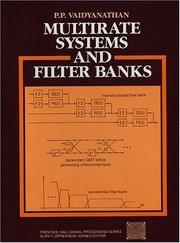
The authoritative and mathematically complete treatment of multirate DSP, polyphase decomposition, and perfect-reconstruction filter banks — indispensable for codec design and modern DSP architectures.

Bridges classical filter theory and modern statistical/adaptive methods with exceptional mathematical rigor, filling gaps left by Oppenheim and preparing the reader for statistical signal processing.
Statistical & Adaptive Signal Processing
ExpertCommand the statistical foundations of DSP — optimal filtering, Wiener and Kalman filters, adaptive algorithms (LMS, RLS), and their convergence properties.
▸ Study plan for this stage
Pace: 8–10 weeks, ~40–50 pages/day (Hayes: 4–5 weeks, ~40 pages/day; Haykin: 4–5 weeks, ~50 pages/day)
- Statistical signal modeling: AR, MA, and ARMA processes; Yule-Walker equations and autocorrelation methods for parameter estimation
- Optimal filtering theory: Wiener filter derivation, normal equations, and the orthogonality principle for minimum mean-square error
- Kalman filtering: state-space models, recursive prediction and update equations, and optimal estimation under linear Gaussian assumptions
- Adaptive filtering fundamentals: cost functions, gradient descent, and the concept of convergence in stationary and non-stationary environments
- LMS (Least Mean Squares) algorithm: update rule, convergence conditions, step-size selection, and stability analysis
- RLS (Recursive Least Squares) algorithm: exponential weighting, forgetting factor, computational efficiency, and tracking performance
- Convergence analysis: mean convergence, mean-square convergence, excess mean-square error, and misadjustment in adaptive algorithms
- Applications and trade-offs: computational complexity, convergence speed, tracking ability, and robustness in real-world adaptive filtering scenarios
- How do you derive the Wiener filter, and what does the orthogonality principle tell you about its optimality?
- What are the differences between AR, MA, and ARMA models, and how do you estimate their parameters using autocorrelation methods?
- Explain the state-space formulation of the Kalman filter and derive the prediction and update equations from first principles.
- Compare the LMS and RLS algorithms: what are their update rules, convergence properties, and computational costs?
- How do you select the step size in LMS to balance convergence speed and stability, and what is the relationship to eigenvalues of the autocorrelation matrix?
- What is the forgetting factor in RLS, and how does it enable tracking of time-varying systems?
- Define mean convergence, mean-square convergence, and excess mean-square error; how do they relate to the misadjustment of an adaptive filter?
- When would you choose Kalman filtering over Wiener filtering, and what assumptions must hold for each to be optimal?
- Implement the Wiener filter for a noise-reduction problem: derive the normal equations, compute the optimal coefficients, and compare against a fixed FIR filter.
- Estimate AR, MA, and ARMA model parameters from a synthetic time series using Yule-Walker and least-squares methods; validate by generating synthetic data from the fitted models.
- Simulate a Kalman filter for a simple tracking problem (e.g., position/velocity estimation with noisy measurements); plot state estimates and compare with ground truth.
- Implement the LMS algorithm for adaptive channel equalization or system identification; vary the step size and observe convergence behavior and steady-state error.
- Implement the RLS algorithm for the same problem as LMS; compare convergence speed, computational cost, and tracking ability with different forgetting factors.
- Analyze convergence of LMS theoretically: compute eigenvalues of the autocorrelation matrix, determine step-size bounds, and verify predictions against simulation.
- Design an adaptive filter to cancel narrowband interference in a signal; use LMS or RLS and measure performance (SNR improvement, convergence time) under stationary and non-stationary conditions.
- Implement a Kalman filter with time-varying process and measurement noise; test robustness to model mismatch and compare with a fixed Wiener filter.
Next up: Mastery of statistical and adaptive signal processing foundations—optimal filtering, Kalman filtering, and adaptive algorithms—prepares you to tackle advanced topics such as spectral estimation, multirate signal processing, or application-specific domains (e.g., communications, audio, biomedical) where these techniques are deployed in practice.

A rigorous and well-organized graduate text covering power spectra, optimal Wiener filtering, Kalman filtering, and parametric spectral estimation — the ideal entry point into statistical DSP.
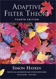
The definitive reference on adaptive filtering: LMS, RLS, Kalman-based adaptive filters, and convergence analysis. Reading Hayes first ensures the statistical background needed to absorb Haykin's depth.
Research-Grade Depth
ExpertEngage with the mathematical frontier of DSP — sparse representations, compressed sensing, wavelets, and time-frequency analysis — enabling original research and cutting-edge system design.
▸ Study plan for this stage
Pace: 8–10 weeks, ~40–50 pages/day (with 2–3 days per week for deep mathematical work and implementation)
- Wavelet decomposition and multiresolution analysis: constructing orthogonal and biorthogonal wavelets, scaling functions, and filter banks for hierarchical signal representation
- Time-frequency localization: understanding the uncertainty principle, Gabor frames, and wavelet packets as tools for joint time-frequency analysis superior to Fourier methods
- Sparse signal representations: exploiting sparsity in wavelet and dictionary domains to achieve compression, denoising, and feature extraction with minimal coefficients
- Compressed sensing theory: recovery of sparse signals from far fewer measurements than Nyquist rate via convex optimization (L1 minimization) and coherence conditions
- Incoherence and restricted isometry property (RIP): mathematical foundations ensuring stable recovery from undersampled data in compressed sensing
- Practical algorithms: matching pursuit, basis pursuit, iterative thresholding, and greedy methods for sparse approximation and signal reconstruction
- Applications to real-world systems: image denoising, compression, feature extraction, and sensor design using wavelet and compressed sensing frameworks
- How do wavelets achieve better time-frequency localization than the Fourier transform, and what is the mathematical relationship between scaling functions and wavelet functions?
- What conditions (incoherence, RIP) must a measurement matrix satisfy for compressed sensing to guarantee stable recovery of sparse signals, and why is L1 minimization the right convex relaxation?
- How do you construct an orthogonal wavelet filter bank, and what role do the Daubechies conditions play in ensuring perfect reconstruction?
- Compare matching pursuit, basis pursuit, and iterative thresholding: when is each method appropriate, and what are their convergence guarantees?
- How would you design a compressed sensing system for a specific application (e.g., MRI, radar, or imaging), and what trade-offs exist between measurement cost and reconstruction quality?
- What is the connection between wavelet sparsity and the success of compressed sensing, and how do you exploit this in practice?
- Implement a discrete wavelet transform (DWT) using Daubechies filters from scratch; verify perfect reconstruction and measure energy compaction on real signals (audio, images)
- Construct a wavelet packet decomposition tree and compare its time-frequency tiling to the standard wavelet decomposition; apply to a chirp or multi-component signal
- Solve a compressed sensing recovery problem using CVX or CVXPY: design a random Gaussian measurement matrix, subsample a sparse signal, and recover it via L1 minimization; plot phase transitions
- Implement matching pursuit and basis pursuit algorithms; compare convergence speed and approximation error on a signal with known sparse representation
- Analyze the coherence and RIP of a measurement matrix; compute bounds on the number of measurements needed for guaranteed recovery of k-sparse signals
- Design and simulate a compressed sensing imaging system (e.g., single-pixel camera or MRI undersampling); reconstruct images from 30–50% of Fourier coefficients and evaluate quality metrics (PSNR, SSIM)
Next up: This stage equips you with the mathematical and algorithmic tools to understand and design cutting-edge signal processing systems; the next stage will focus on translating these theoretical foundations into practical, production-grade implementations and domain-specific applications (e.g., deep learning, real-time systems, or specialized hardware).
The masterwork on wavelets, sparse representations, and time-frequency analysis by one of the field's founders; it unifies filter banks, frames, and compressed sensing into a single coherent mathematical vision.

A rigorous, edited volume covering the theory of sparse recovery, RIP conditions, and practical algorithms — the essential reference for the modern intersection of DSP, optimization, and machine learning.
Discussion
Keep reading
Paths that share books, cover the same subject, or open a related topic.