Multivariable calculus: a reading path beyond one dimension
This curriculum builds a deep mastery of multivariable calculus across three tightly sequenced stages, starting from a solid single-variable foundation and advancing through rigorous vector calculus and its classical integral theorems. Each stage sharpens both geometric intuition and analytical precision, so that by the end the reader can fluently work with partial derivatives, gradients, multiple integrals, and the theorems of Green, Stokes, and Gauss in both computational and proof-based settings.
Bridging the Gap: Single to Multivariable
IntermediateRefresh and extend single-variable intuition into multiple dimensions — coordinates, limits, partial derivatives, and the geometry of surfaces — so that every later concept has a concrete mental picture.
▸ Study plan for this stage
Pace: 4–5 weeks, ~25–30 pages/day (Stewart chapters 12–14, then Schey chapters 1–3). Allocate 2–3 weeks to Stewart's foundational material, then 1–2 weeks to Schey's geometric intuition.
- 3D coordinate systems and vectors as geometric objects with magnitude and direction
- Limits and continuity in multiple dimensions — why ε-δ definitions extend naturally
- Partial derivatives as directional rates of change and the geometry of tangent planes
- Gradient vector as the direction of steepest ascent and its role in optimization
- Level curves and surfaces as visual tools for understanding multivariable functions
- The Jacobian matrix as a linear approximation of multivariable functions
- Div, grad, and curl as differential operators encoding physical meaning (flux, flow, rotation)
- How do you interpret a partial derivative ∂f/∂x geometrically, and why is it different from the total derivative df/dx in single-variable calculus?
- Given a surface z = f(x,y), how do level curves and the gradient vector relate, and what does the gradient tell you about the surface's behavior?
- What is the Jacobian matrix, and how does it generalize the derivative to vector-valued functions of multiple variables?
- How do divergence, gradient, and curl differ in meaning, and what physical phenomena does each one describe?
- Why does the chain rule in multivariable calculus require matrix multiplication, and how does this connect to linear approximation?
- How would you use partial derivatives and the gradient to find and classify critical points of a multivariable function?
- Plot level curves for functions like z = x² + y², z = x² − y², and z = sin(x)cos(y) by hand; verify that the gradient is perpendicular to level curves.
- Compute partial derivatives for 5–7 functions (polynomial, exponential, trigonometric) and sketch the tangent plane at a given point.
- Given a vector field F(x,y) = (P(x,y), Q(x,y)), compute ∇·F (divergence) and ∇×F (curl in 2D) for 3–4 examples; interpret the results physically.
- Use the chain rule to differentiate composite functions like f(g(x,y), h(x,y)) and verify your answer by direct substitution.
- Find critical points of a multivariable function using ∇f = 0, compute the Hessian, and classify them as local maxima, minima, or saddle points.
- Sketch a vector field (e.g., F = (x, y) or F = (−y, x)) and identify regions of positive/negative divergence and rotation by visual inspection.
Next up: This stage establishes the geometric intuition and computational fluency with partial derivatives, gradients, and vector calculus operators that are essential for the next stage's focus on integration in multiple dimensions (double and triple integrals, line and surface integrals) and the fundamental theorems (Green's, Stokes', divergence theorem).

Stewart's chapters on multivariable calculus (Chapters 12–16) are the most widely used bridge from single-variable work, offering clear explanations of partial derivatives, gradients, and double/triple integrals with abundant worked examples. Starting here ensures no gaps in computational fluency before moving to more rigorous texts.
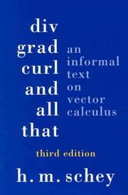
This slim, physics-motivated book builds vivid geometric intuition for gradient, divergence, and curl — exactly the vocabulary needed to make sense of vector fields and the integral theorems. Reading it alongside Stewart cements the 'why' behind the symbols.
Core Multivariable Calculus: Depth and Rigor
IntermediateDevelop a thorough, rigorous command of partial derivatives, the chain rule, optimization with Lagrange multipliers, multiple integrals with change of variables, and line and surface integrals — the full computational and conceptual toolkit.
▸ Study plan for this stage
Pace: 12–14 weeks, ~40–50 pages/day (Stewart: 6–7 weeks, ~45 pages/day; Marsden: 3–4 weeks, ~40 pages/day; Spivak: 2–3 weeks, ~35 pages/day for depth and proof mastery)
- Partial derivatives, directional derivatives, and the gradient as a vector of rates of change
- The multivariable chain rule in all forms (tree diagrams, matrix Jacobians, composition rules)
- Critical points, Hessian matrices, and the second derivative test for local extrema
- Constrained optimization via Lagrange multipliers and the geometric interpretation of the constraint
- Double and triple integrals, Fubini's theorem, and integration order selection
- Change of variables in multiple integrals: Jacobian determinants and polar, cylindrical, spherical coordinates
- Line integrals of scalar and vector fields, path independence, and conservative fields
- Surface integrals, flux, and the divergence and curl operators
- Green's, Stokes', and the divergence theorem as unified statements about boundary behavior
- Rigorous proofs of key theorems and the role of differentiability, compactness, and continuity assumptions
- How do you compute the gradient of a multivariable function, and what does it represent geometrically and physically?
- State and apply the chain rule for a composite function of several variables; explain the role of the Jacobian matrix.
- Given a function on a compact domain, how do you find and classify all critical points (local max, min, saddle)?
- How do Lagrange multipliers work, and why does the condition ∇f = λ∇g characterize constrained extrema?
- Compute a double or triple integral by choosing an appropriate order of integration and coordinate system.
- Given a change of variables, how do you compute the Jacobian and apply it to transform an integral?
- What is the difference between a conservative vector field and a path-dependent one, and how do you test for conservatism?
- State Green's theorem, Stokes' theorem, and the divergence theorem; apply each to compute a line or surface integral.
- Stewart Ch. 14–15: Compute partial derivatives and gradients for 10+ functions; sketch level curves and gradient vectors.
- Stewart Ch. 14: Use the chain rule (tree diagrams) to find dz/dt for 8–10 composite functions; verify with direct substitution.
- Stewart Ch. 14: Find and classify critical points of 6–8 functions using the Hessian; identify saddle points, local maxima, minima.
- Stewart Ch. 14: Solve 8–10 constrained optimization problems (e.g., maximize volume subject to surface area constraint) using Lagrange multipliers.
- Stewart Ch. 15: Evaluate 10+ double integrals by choosing optimal integration order; sketch regions of integration.
- Stewart Ch. 15: Compute 8–10 integrals using polar, cylindrical, and spherical coordinates; justify coordinate choice.
- Marsden Ch. 2–3: Verify path independence for 5–6 vector fields; compute line integrals using potential functions.
- Marsden Ch. 4: Apply Green's theorem to compute 6–8 line integrals as double integrals; verify both methods.
Next up: Mastery of partial derivatives, chain rules, optimization, multiple integrals, and the classical integral theorems (Green's, Stokes', divergence) provides the rigorous computational foundation and geometric intuition needed to move into advanced topics such as differential forms, manifold theory, tensor calculus, or specialized applications (PDEs, fluid dynamics, electromagnetism).

The standalone multivariable volume of Stewart lets the reader focus exclusively on Chapters 12–16 at a deliberate pace, reinforcing every technique — from the gradient and directional derivatives to Green's and Stokes' theorems — with a large problem set.
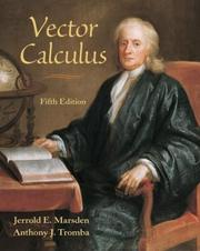
Marsden and Tromba's classic text elevates the treatment with cleaner mathematical language, stronger geometric reasoning, and careful statements of Green's, Stokes', and the Divergence theorems. It is the standard bridge between computational calculus and real analysis.

Spivak's concise masterpiece re-derives all of multivariable calculus from first principles — inverse and implicit function theorems, differential forms, and a unified Stokes' theorem. Reading it after Marsden reveals the deep structure underlying every formula encountered so far.
Advanced Perspectives: Analysis and Differential Forms
ExpertUnderstand multivariable calculus as a chapter of real analysis and differential geometry — mastering the implicit and inverse function theorems, differential forms, and the general Stokes' theorem — achieving the deepest possible conceptual understanding.
▸ Study plan for this stage
Pace: 8–10 weeks, ~40–50 pages/day (with 2–3 days per week for problem-solving and integration)
- Manifolds as geometric objects: definition, tangent spaces, and smooth maps between manifolds
- Implicit and Inverse Function Theorems: precise statements, proofs, and applications to constrained optimization and local diffeomorphisms
- Differential forms as antisymmetric multilinear functionals: wedge product, exterior derivative, and their geometric meaning
- Integration of differential forms: pullback of forms, change of variables, and Stokes' theorem in its general coordinate-free form
- The general Stokes' theorem as unification: how it encompasses divergence theorem, curl theorem, and classical Green's theorem
- Real analysis foundations for multivariable calculus: uniform continuity, compactness, and the inverse function theorem's role in local invertibility
- Differential geometry perspective: how differential forms encode geometric and analytic information on manifolds
- Cohomology and closed vs. exact forms: understanding when line integrals are path-independent and topological obstructions
- State the Implicit Function Theorem precisely and explain why the non-vanishing of a Jacobian determinant is both necessary and sufficient for local invertibility.
- What is a differential form, and how does the wedge product encode orientation and dimensionality? Why is the exterior derivative the natural notion of 'derivative' for forms?
- Prove or carefully explain why d(dω) = 0 for any differential form ω, and what this means geometrically.
- State the general Stokes' theorem and show how the divergence theorem and classical Stokes' theorem emerge as special cases.
- What is the relationship between closed forms (dω = 0) and exact forms (ω = dη)? Give an example of a closed form that is not exact.
- How does the pullback of a differential form under a smooth map work, and why is it natural for integration?
- Explain the role of manifolds with boundary in the statement of Stokes' theorem, and why the boundary operator ∂ satisfies ∂(∂M) = ∅.
- What does it mean for a vector field to be conservative, and how is this captured by the language of differential forms and cohomology?
- From Munkres: Work through all problems in Chapters 1–2 (manifolds and smooth maps) to build geometric intuition; pay special attention to constructing explicit examples of manifolds (spheres, tori, projective spaces) and verifying smoothness.
- From Munkres: Complete the full proof of the Inverse Function Theorem (Chapter 3) by hand, then apply it to prove that the set of invertible n×n matrices is an open manifold.
- From Hubbard: Work all computational exercises on wedge products and exterior derivatives (Chapter 1) to develop fluency; compute dω for several explicit 1-forms and 2-forms on ℝ³.
- From Hubbard: Verify Stokes' theorem for at least three explicit examples: a 1-form integrated over a curve, a 2-form over a surface, and a 3-form over a solid region.
- Prove that if ω is a closed 1-form on a simply connected domain, then ω is exact, and use this to characterize conservative vector fields.
- Construct a closed 2-form on ℝ³ \ {origin} that is not exact (e.g., the solid angle form), and explain why it detects the topological obstruction.
- From Munkres: Solve problems on the Implicit Function Theorem to practice identifying when level sets are manifolds and computing their tangent spaces.
- From Hubbard: Work through the pullback exercises to internalize how differential forms transform under smooth maps; verify the chain rule for exterior derivatives under pullback.
Next up: This stage equips you with the rigorous, coordinate-free language of differential forms and manifolds—the foundation for studying advanced topics such as Riemannian geometry, Lie groups, algebraic topology, or applications to physics (electromagnetism, fluid dynamics, general relativity).

Munkres provides the most reader-friendly rigorous treatment of multivariable analysis, filling every gap left by Spivak with detailed proofs and motivation. It is the ideal next step for solidifying the inverse/implicit function theorems and integration on chains.
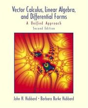
Hubbard unifies linear algebra, multivariable calculus, and differential forms into one coherent framework, making the relationship between the classical integral theorems and the general Stokes' theorem completely transparent. This book is the capstone that ties every prior stage together.
Discussion
Keep reading
Paths that share books, cover the same subject, or open a related topic.