Electromagnetism reading path: from fields to Maxwell's equations
This curriculum takes an intermediate physics student from a solid grounding in electrostatics and magnetostatics all the way to a unified, mathematically rigorous understanding of electromagnetic waves and Maxwell's equations. Each stage builds directly on the last — intuition and physical reasoning come first, vector calculus and field theory deepen in the middle stages, and the final stage delivers the full theoretical and advanced treatment that connects electromagnetism to optics, relativity, and modern physics.
Foundations & Physical Intuition
IntermediateEstablish a confident physical picture of electric and magnetic fields, Coulomb's law, Gauss's law, and the Biot–Savart law, with enough mathematical fluency to move into vector calculus treatments.
▸ Study plan for this stage
Pace: 8–10 weeks, ~40–50 pages/day (Sears first, then Feynman). Sears chapters on electrostatics and magnetism (~400 pages) over 5–6 weeks; Feynman Vol. 2 chapters 1–7 (~300 pages) over 3–4 weeks for conceptual reinforcement and intuition-building.
- Electric charge, quantization, and conservation; Coulomb's law as the fundamental force law between point charges
- Electric field as a vector quantity: definition, superposition, and physical interpretation as the force per unit charge
- Gauss's law: mathematical statement, physical meaning, and application to symmetric charge distributions (spheres, cylinders, planes)
- Magnetic force on moving charges and current-carrying conductors; the Lorentz force law
- Biot–Savart law: calculating magnetic fields from current distributions; symmetry arguments to simplify calculations
- Relationship between current, charge motion, and magnetic field generation; magnetic dipoles and their behavior
- Flux concepts: electric flux and Gauss's law; magnetic flux and its conservation (no magnetic monopoles)
- Vector field visualization and intuition: field lines, field strength, and how sources (charges/currents) create fields
- State Coulomb's law and explain what each term represents. How does the electric field of a point charge follow from it?
- Derive the electric field at distance r from an infinite uniformly charged plane using Gauss's law. Why is Gauss's law more efficient than Coulomb's law here?
- A uniformly charged sphere of radius R contains total charge Q. Use Gauss's law to find the electric field both inside (r < R) and outside (r > R) the sphere.
- State the Biot–Savart law and use it to find the magnetic field at the center of a circular current loop of radius a carrying current I.
- Explain the Lorentz force law. How does it differ from Coulomb's law, and why does a stationary charge experience no magnetic force?
- What is the physical meaning of 'no magnetic monopoles'? How does this relate to Gauss's law for magnetism?
- Solve 5–6 Coulomb's law problems from Sears (point charges, superposition) to build fluency with vector addition and field superposition.
- Apply Gauss's law to at least 4 symmetric geometries (infinite plane, infinite line, sphere, cylinder) from Sears; sketch the Gaussian surfaces and explain your choice.
- Calculate the electric field inside and outside a uniformly charged sphere; verify continuity at the boundary.
- Work through Feynman's conceptual examples on electric fields (Vol. 2, Ch. 4–5); reproduce his field-line sketches for simple charge configurations.
- Solve 4–5 Biot–Savart problems: straight wire, circular loop, solenoid. Sketch the resulting field patterns and identify symmetries.
- Solve a mixed problem: given a charge distribution, use Gauss's law to find E; given a current distribution, use Biot–Savart to find B. Compare the mathematical structures.
- Create a visual summary (hand-drawn or digital) showing how Coulomb's law, Gauss's law, and Biot–Savart law are related; annotate with physical intuition from Feynman.
Next up: This stage builds the physical intuition and mathematical competence needed to transition to the differential form of Maxwell's equations and vector calculus treatments, where Gauss's law becomes ∇·E and the Biot–Savart law emerges from ∇×B, unifying electromagnetism into a coherent mathematical framework.

A rigorous but accessible starting point that covers electrostatics, circuits, magnetism, and induction with clear diagrams and worked examples — ideal for cementing the physical intuition needed before tackling field theory.
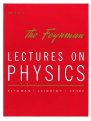
Feynman's legendary treatment of electromagnetism builds deep physical insight into fields, potentials, and Maxwell's equations through vivid reasoning; read this second to reframe and enrich what Young introduced.
Core Electromagnetism with Vector Calculus
IntermediateMaster electric and magnetic fields, scalar and vector potentials, boundary conditions, and Maxwell's equations in both integral and differential form using the full machinery of vector calculus.
▸ Study plan for this stage
Pace: 12–14 weeks, ~40–50 pages/day (Griffiths first 8–9 weeks, then Schey 3–4 weeks for reinforcement and depth)
- Electric field as a vector field: definition, superposition, and physical interpretation of field lines and flux
- Gauss's law in integral and differential form (∇·E = ρ/ε₀) and its application to symmetric charge distributions
- Scalar potential φ and the relationship E = −∇φ; solving Laplace's and Poisson's equations
- Magnetic field B, Ampère's law in integral and differential form (∇×B = μ₀J), and the Biot–Savart law
- Vector potential A and the relationship B = ∇×A; gauge freedom and the Coulomb gauge
- Faraday's law in integral and differential form (∇×E = −∂B/∂t) and electromagnetic induction
- Displacement field D and auxiliary field H; boundary conditions for E, B, D, H at material interfaces
- Maxwell's equations as a unified system in both integral and differential forms; wave equation and electromagnetic waves
- Divergence, gradient, and curl operators: geometric meaning, Cartesian and curvilinear coordinates, and integral theorems (Gauss, Stokes)
- State Maxwell's four equations in both integral and differential form, and explain the physical meaning of each term.
- Derive the electric field of an infinite uniformly charged plane and a uniformly charged sphere using Gauss's law; verify your results using the scalar potential.
- Given a current distribution J(r), explain how to find the magnetic field using both Ampère's law and the Biot–Savart law, and discuss when each approach is practical.
- What are boundary conditions for the tangential and normal components of E, B, D, and H at an interface between two media? Derive them from Maxwell's equations.
- Explain the relationship between the vector potential A and magnetic field B; why is gauge freedom important, and what does the Coulomb gauge accomplish?
- Derive Faraday's law in differential form from the integral form, and explain how a changing magnetic flux induces an electric field.
- How do the divergence, gradient, and curl operators relate to physical quantities (flux, potential, circulation)? Compute these operators in Cartesian and cylindrical coordinates.
- Starting from Maxwell's equations in vacuum, derive the wave equation for E and B, and show that electromagnetic waves propagate at speed c.
- Work through Griffiths Chapters 2–3 end-of-chapter problems (at least 15–20 problems) on Gauss's law, electric potential, and energy; focus on problems requiring both integral and differential approaches.
- Solve 10–12 problems from Griffiths Chapter 5 on magnetic fields, Ampère's law, and the Biot–Savart law; include at least 3 problems with non-trivial symmetries (e.g., solenoids, toroidal coils).
- Derive boundary conditions for E, B, D, H from first principles using Maxwell's equations and small Gaussian pillboxes or Amperian loops; then apply them to 5–6 problems involving dielectric or magnetic interfaces.
- Work through Schey's chapters on div, grad, and curl (Chapters 2–4): compute these operators in Cartesian, cylindrical, and spherical coordinates for at least 8–10 scalar and vector fields; verify results numerically or graphically.
- Solve 8–10 problems involving the vector potential A: compute A from a given current distribution, verify B = ∇×A, and explore gauge transformations.
- Complete 6–8 problems on Faraday's law and electromagnetic induction (Griffiths Chapter 3); include motional emf, changing flux, and mutual inductance.
- Prove the integral theorems (divergence theorem, Stokes' theorem) using Schey's geometric approach; apply them to 4–5 problems to verify Maxwell's equations in integral form.
- Solve the wave equation for E and B in vacuum and in simple media (e.g., good conductors); compute phase velocity, wavelength, and attenuation for at least 3 different scenarios.
Next up: This stage provides the complete mathematical and conceptual foundation—Maxwell's equations, vector calculus, and boundary conditions—needed to tackle advanced topics such as electromagnetic radiation, waveguides, antennas, and relativistic formulations of electromagnetism in the next stage.

The definitive undergraduate text: it builds from Coulomb's law through potentials, dielectrics, magnetic materials, and Maxwell's equations with exceptional clarity — the essential backbone of this curriculum.
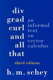
A concise, physics-motivated guide to vector calculus that should be read alongside or just before Griffiths to ensure the mathematical tools (divergence theorem, Stokes' theorem) feel natural rather than mechanical.
Electromagnetic Waves & Radiation
IntermediateUnderstand how Maxwell's equations predict electromagnetic waves, derive wave propagation in media, and describe radiation from accelerating charges and antennas.
▸ Study plan for this stage
Pace: 8–10 weeks, ~40–50 pages/week (approximately 5–7 pages/day with 2 days off)
- Maxwell's equations as the foundation for electromagnetic wave existence and their physical interpretation
- Derivation of the wave equation from Maxwell's equations in free space and in conducting/dielectric media
- Plane wave solutions: amplitude, phase velocity, wavelength, frequency, and polarization
- Energy transport and the Poynting vector as a measure of electromagnetic power flow
- Boundary conditions and reflection/transmission of waves at interfaces between media
- Radiation from accelerating charges: the relationship between acceleration and electromagnetic field generation
- Antenna theory: dipole radiation patterns, radiation resistance, and directivity
- Propagation in dispersive and lossy media: attenuation, phase velocity, and group velocity
- How do Maxwell's equations lead to the prediction of electromagnetic waves, and what role does the displacement current play?
- Derive the wave equation for the electric field in free space starting from Maxwell's equations, and identify the wave speed.
- What is a plane wave solution to Maxwell's equations, and how are amplitude, wavelength, frequency, and polarization defined?
- Explain the Poynting vector and how it describes energy flow in an electromagnetic wave.
- How do electromagnetic waves behave at the boundary between two media, and what determines the reflection and transmission coefficients?
- Why does an accelerating charge radiate electromagnetic waves, and how does the radiated power depend on acceleration?
- Describe the radiation pattern of an oscillating electric dipole and explain the concept of radiation resistance.
- How do electromagnetic waves propagate differently in conducting versus dielectric media, and what is the skin depth?
- Work through the complete derivation of the wave equation from Maxwell's equations; verify each step and confirm the wave speed equals c in free space.
- Solve for plane wave solutions (E and B fields) in free space; practice writing solutions in both real and complex notation.
- Calculate the Poynting vector for a given plane wave and verify that it points in the direction of propagation with magnitude equal to the intensity.
- Apply boundary conditions at a dielectric interface to find reflection and transmission coefficients for normal and oblique incidence.
- Derive the electric and magnetic fields radiated by an oscillating dipole; sketch the radiation pattern and calculate the total radiated power.
- Compute the radiation resistance of a short dipole antenna and relate it to the input impedance.
- Analyze wave propagation in a lossy conductor: calculate the skin depth for a given frequency and conductivity, and sketch the field decay.
- Work a complete problem involving antenna design: specify dimensions, calculate resonant frequency, and estimate the radiation pattern for a given application.
Next up: This stage establishes the physical and mathematical foundation for understanding how electromagnetic energy propagates and radiates, preparing you to explore practical applications such as waveguides, transmission lines, and antenna arrays in the next stage.
Bridges the gap between field theory and practical wave propagation, antennas, and transmission lines, providing engineering-grounded depth that complements Griffiths' theoretical approach.
Graduate-Level Field Theory
ExpertAchieve a complete, rigorous graduate-level command of classical electrodynamics including Green's functions, multipole expansions, relativistic formulation, and radiation reaction.
▸ Study plan for this stage
Pace: 12–14 weeks, ~40–50 pages/day (Jackson: 8–9 weeks; Landau: 3–4 weeks). Allocate 2–3 days per chapter for problem-solving and integration.
- Green's functions and their role in solving inhomogeneous Maxwell equations (Jackson Ch. 1–3)
- Multipole expansions: electric, magnetic, and radiation multipole moments (Jackson Ch. 4–5)
- Radiation from accelerated charges and dipole radiation (Jackson Ch. 9)
- Relativistic formulation of electrodynamics: four-vectors, covariant Maxwell equations, and Lorentz transformations (Jackson Ch. 11–12; Landau Ch. 1–2)
- Radiation reaction and self-energy: Abraham–Lorentz equation and its physical interpretation (Jackson Ch. 16; Landau Ch. 8)
- Lagrangian and Hamiltonian formulations in field theory and their gauge structure (Landau Ch. 1–3)
- Electromagnetic energy-momentum tensor and conservation laws (Jackson Ch. 6; Landau Ch. 1)
- Scattering and diffraction: formal scattering theory and optical theorem (Jackson Ch. 10)
- Derive the retarded Green's function for the wave equation and explain how it encodes causality in electromagnetic problems.
- Calculate the electric and magnetic dipole moments for a localized charge and current distribution, and determine the leading multipole contribution to the far field.
- Starting from the Liénard–Wiechert potentials, derive the power radiated by an accelerated point charge and express it in terms of acceleration.
- Write Maxwell's equations in covariant form using four-vectors and the electromagnetic field tensor, and show how Lorentz transformations mix electric and magnetic fields.
- Explain the physical meaning and limitations of the Abraham–Lorentz equation, including the runaway solution problem and its resolution.
- Construct the energy-momentum tensor for the electromagnetic field and derive the Poynting vector and Maxwell stress tensor from it.
- For a given charge distribution and radiation multipole order, estimate the relative importance of different multipole contributions to the radiated power.
- Explain how gauge invariance constrains the form of the electromagnetic Lagrangian and why it is essential for consistency in quantum field theory.
- Jackson Ch. 1–3: Solve 5–6 problems on Green's functions (e.g., 1.1, 1.4, 2.1, 3.1, 3.5) to master boundary value problems and causality.
- Jackson Ch. 4–5: Work through multipole expansion problems (e.g., 4.1, 4.3, 5.1, 5.2) for both static and dynamic cases; compute dipole and quadrupole moments for simple geometries.
- Jackson Ch. 9: Solve radiation problems (e.g., 9.1, 9.2, 9.3, 9.5) including dipole, quadrupole, and magnetic dipole radiation; calculate power for oscillating charges.
- Jackson Ch. 11–12: Work through relativistic formulation problems (e.g., 11.1, 11.3, 12.1, 12.2) to verify covariance and Lorentz transformations of fields.
- Jackson Ch. 16: Solve problems on radiation reaction (e.g., 16.1, 16.2) and discuss the physical interpretation of the Abraham–Lorentz equation.
- Landau Ch. 1–3: Derive the Lagrangian and Hamiltonian for the electromagnetic field; verify gauge invariance and conservation laws from the action principle.
- Landau Ch. 8: Work through radiation reaction problems in the Landau formalism; compare results with Jackson's treatment.
- Comprehensive problem: Given a time-varying charge and current distribution (e.g., oscillating dipole or synchrotron radiation), compute the full multipole expansion, identify dominant contributions, and calculate total radiated power using both Jackson and Landau approaches.
Next up: Mastery of classical field theory, covariance, and radiation reaction provides the mathematical and conceptual foundation for quantum field theory, where the same Green's functions, Lagrangian formalism, and gauge principles govern the quantized electromagnetic field and its interactions with matter.

The canonical graduate reference — exhaustive, mathematically demanding, and comprehensive. After Griffiths, Jackson's depth on boundary-value problems, multipoles, and radiation is the natural next summit.
Landau and Lifshitz's elegant, terse treatment unifies electromagnetism with special relativity through the action principle, offering a profoundly different and complementary perspective to Jackson's approach.
Discussion
Keep reading
Paths that share books, cover the same subject, or open a related topic.