Fluid dynamics reading path: from flow basics to Navier-Stokes
This curriculum takes an intermediate learner from a solid grounding in fluid statics and kinematics through the mathematical heart of fluid dynamics — viscosity, the Navier-Stokes equations, and turbulence — and finally into the computational and modeling tools used to simulate real fluid behavior. Each stage builds the vocabulary, physical intuition, and mathematical machinery needed for the next, ensuring no conceptual gaps along the way.
Foundations & Physical Intuition
IntermediateEstablish a firm physical picture of fluid properties — pressure, viscosity, density, and flow regimes — and develop intuition for how and why fluids move before tackling heavy mathematics.
▸ Study plan for this stage
Pace: 4–5 weeks, ~40–50 pages/day (White: Chapters 1–3, ~150 pages; Batchelor: Chapters 1–2, ~80 pages)
- Fluid properties (density, viscosity, surface tension, bulk modulus) and how they vary with temperature and pressure
- Pressure as a normal stress and its role in hydrostatic equilibrium and fluid motion
- Viscosity (dynamic and kinematic) as resistance to shear deformation; Newtonian vs. non-Newtonian fluids
- Flow regimes: laminar vs. turbulent, characterized by Reynolds number and physical transitions
- Continuum hypothesis and the Eulerian vs. Lagrangian descriptions of fluid motion
- Kinematics of fluid flow: streamlines, pathlines, streaklines, and the velocity field as a primary descriptor
- Strain rate and vorticity as measures of deformation and rotation in a fluid element
- Intuitive understanding of why pressure gradients and viscous stresses drive fluid motion
- What is viscosity, how is it measured, and why do some fluids (like honey) have much higher viscosity than others (like water)?
- Explain the physical difference between laminar and turbulent flow, and describe the role of Reynolds number in determining which regime occurs.
- What is the continuum hypothesis, and under what conditions is it valid? Why is it important for fluid mechanics?
- Describe the difference between Eulerian and Lagrangian descriptions of fluid flow, and give an example of when each perspective is useful.
- What are streamlines, pathlines, and streaklines? How do they relate to one another in steady vs. unsteady flow?
- Why does a pressure gradient cause fluid to accelerate, and how is this related to the concept of a body force?
- Measure the viscosity of common fluids (water, oil, honey, glycerin) using a simple falling-ball or capillary tube method; plot viscosity vs. temperature and compare to published data.
- Sketch velocity profiles and streamline patterns for flow in a pipe, flow around a cylinder, and flow between parallel plates; identify regions of high shear rate.
- Calculate Reynolds numbers for everyday flows (water flowing from a faucet, air around a moving car, blood in an artery) and predict whether each is laminar or turbulent.
- Using White's examples, work through pressure distribution problems in static fluids (manometers, hydrostatic pressure in a tank) to build intuition for pressure gradients.
- Create a simple flow visualization experiment (e.g., dye in water, smoke in air, or food coloring in a bathtub) and sketch the observed streamlines and vorticity patterns.
- Solve 5–8 problems from White (Chapters 1–3) on fluid properties, hydrostatics, and flow classification to reinforce conceptual understanding.
Next up: This stage equips you with the physical intuition and vocabulary needed to move into the mathematical foundations—the Navier–Stokes equations and conservation laws—which will quantify the relationships between pressure, viscosity, and flow that you now understand qualitatively.
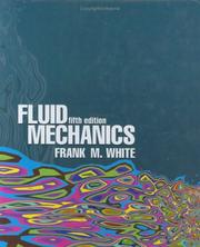
A widely adopted undergraduate-to-graduate bridge text that introduces pressure, viscosity, laminar vs. turbulent flow, and the Reynolds number with clear physical motivation and worked examples — the ideal starting point for an intermediate learner.
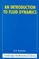
Batchelor's classic provides the rigorous physical and mathematical foundations — including stress tensors, viscosity, and the derivation of the Navier-Stokes equations — that every serious student of fluid dynamics must encounter early.
Core Theory: Viscosity, Laminar Flow & Navier-Stokes
IntermediateDerive and deeply understand the Navier-Stokes equations, solve canonical viscous and laminar flow problems (Couette, Poiseuille, boundary layers), and appreciate the physical meaning of each term.
▸ Study plan for this stage
Pace: 8–10 weeks, ~40–50 pages/day (White: 4–5 weeks; Schlichting: 4–5 weeks)
- Stress tensor and Newtonian fluid constitutive relations: how viscosity links stress to strain rate
- Derivation of the Navier-Stokes equations from conservation of mass and momentum; physical meaning of each term (pressure gradient, viscous diffusion, convection)
- Couette and Poiseuille flows: exact solutions for laminar flow between parallel plates and in pipes; velocity profiles and shear stress distributions
- Boundary layer concept: thin region near walls where viscous effects dominate; separation of scales and asymptotic matching
- Blasius solution and similarity variables: self-similar solutions for laminar boundary layers on flat plates
- Momentum integral equation (von Kármán): practical tool for boundary layer analysis without solving full Navier-Stokes
- Physical interpretation of dimensionless numbers: Reynolds number (ratio of inertial to viscous forces), Prandtl number (momentum vs. thermal diffusion)
- Derive the Navier-Stokes equations from first principles (conservation of mass and momentum) and explain the physical role of each term: pressure gradient, viscous diffusion, and convective acceleration.
- Solve the Couette flow problem (flow between two parallel plates) and Poiseuille flow (flow in a pipe) analytically; sketch velocity and shear stress profiles and relate them to the pressure gradient.
- What is a boundary layer? Why does it form, and what is the physical basis for the assumption that viscous effects are confined to a thin region near the wall?
- State and apply the Blasius solution for laminar boundary layer flow on a flat plate; explain similarity variables and how they reduce the Navier-Stokes equations to an ODE.
- Derive and apply the momentum integral equation (von Kármán equation) to estimate boundary layer thickness and skin friction without solving the full PDE.
- How do Reynolds number and other dimensionless parameters control the relative importance of viscous versus inertial effects? Give examples from canonical flows.
- Work through White's derivation of the Navier-Stokes equations step-by-step; write out the stress tensor and constitutive relation for a Newtonian fluid in your own words.
- Solve Couette and Poiseuille flows by hand: set up the Navier-Stokes equations, apply boundary conditions, integrate, and plot velocity and shear stress profiles. Compare results for different pressure gradients.
- Numerically solve the Blasius equation (using a shooting method or built-in ODE solver in Python/MATLAB) and compute boundary layer thickness δ(x) and skin friction coefficient Cf(x) for a flat plate.
- Apply the von Kármán momentum integral equation to estimate boundary layer growth on a flat plate; compare your integral-based result to the Blasius solution.
- Work through Schlichting's treatment of separation: identify conditions under which adverse pressure gradients cause flow separation; sketch streamlines and pressure distributions.
- Solve a practical problem: estimate the drag force on a flat plate (or cylinder) immersed in a viscous flow using boundary layer theory; validate against experimental data or published correlations.
Next up: This stage equips you with the analytical and physical foundations to tackle turbulent flows, heat and mass transfer in boundary layers, and more complex geometries—all of which build on the Navier-Stokes equations and the boundary layer concept you have now mastered.
Dedicated entirely to viscous effects, this book systematically develops exact and approximate solutions to the Navier-Stokes equations for laminar flows, making it the natural next step after a general fluid mechanics introduction.

The definitive reference on viscous boundary layers — the region where viscosity and the Navier-Stokes equations matter most — providing analytical solutions and physical insight that are essential before studying turbulence.
Turbulence: From Onset to Statistical Description
ExpertUnderstand the transition from laminar to turbulent flow, the physics of turbulent eddies and energy cascades, and the statistical frameworks (Reynolds averaging, closure models) used to describe turbulence.
▸ Study plan for this stage
Pace: 8–10 weeks, ~40–50 pages/day (including re-reading difficult sections and working through derivations)
- Transition to turbulence: stability analysis, bifurcation mechanisms, and the onset of chaotic flow behavior
- Turbulent kinetic energy (TKE) budget: production, dissipation, and transport mechanisms across scales
- Energy cascade and spectral analysis: Kolmogorov's theory, inertial subrange, and energy transfer from large to small scales
- Reynolds decomposition and Reynolds-averaged Navier–Stokes (RANS) equations: separating mean and fluctuating components
- Turbulent stress tensor and the closure problem: why additional equations are needed beyond RANS
- Eddy viscosity models and Boussinesq hypothesis: connecting turbulent stresses to mean flow gradients
- Two-equation closure models (k–ε and k–ω): physical basis, model coefficients, and limitations
- Statistical characterization: probability density functions (PDFs), correlations, and spectral tensors in turbulent flows
- What are the physical mechanisms that trigger the transition from laminar to turbulent flow, and how does linear stability analysis predict this transition?
- Explain the energy cascade concept: how does kinetic energy transfer from large scales to small scales, and what is the significance of the Kolmogorov microscale?
- Why is the closure problem fundamental to turbulence modeling, and what assumptions underlie the Boussinesq eddy viscosity hypothesis?
- Derive and interpret the Reynolds-averaged Navier–Stokes equations and the turbulent kinetic energy budget equation from first principles.
- Compare and contrast k–ε and k–ω closure models: what are their physical bases, typical applications, and known limitations?
- How do statistical descriptions (PDFs, correlations, spectral tensors) characterize turbulent flows, and what information do they provide beyond mean-field quantities?
- Work through Pope's derivations of Reynolds decomposition and RANS equations step-by-step; verify dimensional consistency and physical interpretation of each term in the TKE budget.
- Solve linear stability analysis problems (Orr–Sommerfeld equation or simplified versions) to predict the critical Reynolds number for transition in canonical flows (e.g., plane Poiseuille, Blasius boundary layer).
- Implement a simple k–ε or k–ω model in a 1D or 2D channel flow code; compare predictions against experimental data or DNS results provided in Pope's text.
- Analyze turbulent energy spectra from experimental or DNS data: identify the inertial subrange, estimate Kolmogorov scales, and verify Kolmogorov's -5/3 law.
- Compute and plot two-point correlations and spectral tensors for a given turbulent velocity field; interpret the results in terms of eddy structure and anisotropy.
- Write a detailed technical summary (3–5 pages) explaining the physical basis of one closure model (k–ε or k–ω) and its limitations; include derivations and a worked example.
Next up: This stage establishes the foundational physics and statistical tools for describing turbulence at the continuum scale, preparing you to explore advanced modeling techniques (LES, DNS, hybrid RANS-LES methods) and applications to complex flows in the next stage.
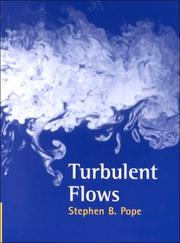
Pope's comprehensive graduate text covers the full arc of turbulence — from instability and transition through Reynolds-averaged equations and closure modeling — and is the canonical modern reference for this stage.
Read alongside or just before Pope, this shorter classic builds physical and scaling intuition for turbulent flows through dimensional reasoning, making Pope's formalism far more digestible.
Modeling & Computational Fluid Dynamics
ExpertTranslate the Navier-Stokes equations into numerical algorithms, understand discretization, stability, and turbulence modeling (RANS, LES), and be able to critically evaluate CFD simulations of real fluid behavior.
▸ Study plan for this stage
Pace: 8–10 weeks, ~40–50 pages/day (mix of theory and worked examples), with 2–3 days per week dedicated to hands-on coding and simulation exercises
- Discretization methods (finite difference, finite volume, finite element) and their application to the Navier-Stokes equations
- Stability analysis, convergence criteria, and the CFL condition in explicit and implicit schemes
- Pressure-velocity coupling algorithms (SIMPLE, SIMPLEC, PISO) for incompressible flow
- Turbulence modeling fundamentals: RANS (k-ε, k-ω models) vs. LES and their computational trade-offs
- Boundary conditions, mesh generation, and grid independence studies in CFD workflows
- Numerical errors: truncation, round-off, and aliasing; how to identify and mitigate them in simulations
- Post-processing, validation, and critical evaluation of CFD results against experimental or analytical benchmarks
- Explain how the finite volume method discretizes the Navier-Stokes equations and why it conserves mass and momentum locally
- What is the CFL condition and why is it essential for stability in explicit time-stepping schemes?
- Describe the SIMPLE algorithm: how does it decouple pressure and velocity, and what are its limitations?
- Compare RANS and LES approaches: what are the computational costs, accuracy trade-offs, and when would you choose one over the other?
- How do you perform a grid independence study, and what does it tell you about the reliability of your CFD simulation?
- What are the main sources of numerical error in CFD, and how can you distinguish between them in a simulation?
- Implement a 1D finite difference solver for the advection-diffusion equation; verify stability against the CFL condition and compare explicit vs. implicit schemes
- Build a 2D finite volume code (or use an open-source framework like OpenFOAM) to simulate laminar flow in a driven cavity; validate against the benchmark solution from Ghia et al.
- Perform a grid independence study on a simple flow case (e.g., flow over a cylinder or channel flow); document how drag coefficient and pressure drop converge with mesh refinement
- Set up and run a RANS simulation (k-ε model) of a turbulent channel or pipe flow; compare wall shear stress and velocity profiles against experimental data or DNS results
- Conduct an LES simulation of the same turbulent flow case and compare computational time, memory usage, and accuracy against the RANS result
- Critically analyze a published CFD paper: identify the discretization method, turbulence model, mesh resolution, boundary conditions, and assess whether the numerical choices are justified and the results are credible
Next up: This stage equips you with the ability to translate continuous fluid equations into discrete, solvable algorithms and to evaluate the fidelity of numerical predictions—essential preparation for specialized topics such as advanced turbulence closure models, multiphase flow simulation, or application-specific CFD (aerodynamics, combustion, heat transfer) in subsequent stages.

A clear, accessible entry into CFD that connects the Navier-Stokes equations directly to finite-volume discretization and turbulence models, bridging the gap between theory and simulation practice.
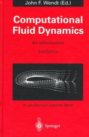
Anderson's text deepens the numerical treatment with a focus on compressible flows and algorithm design, rounding out the curriculum with the tools needed to model a wide range of real fluid phenomena.
Discussion
Keep reading
Paths that share books, cover the same subject, or open a related topic.