Best Books to Learn Remote Sensing and Satellite Image Analysis
Remote sensing is a genuinely technical subject and this path treats it as one. Assume throughout: multivariable calculus, linear algebra including eigen-decomposition, undergraduate probability and statistics, and enough physics to be comfortable with electromagnetic waves, blackbody radiation and Fourier transforms. Some scripting — Python, R or MATLAB — is assumed from stage three onward. The route is deliberately conventional because the field has two textbooks that every degree programme uses and there is no advantage in being clever about it: the standard course first, then the radiative-transfer physics that explains why the numbers mean anything, then digital image processing and classification, then the specialist sensor families, and finally actually doing it on real data. Each entry states what it assumes.
The standard course
BeginnerKnow the electromagnetic spectrum as it is used operationally, the main sensor and platform families, spatial-spectral-radiometric-temporal resolution and the tradeoffs between them, and be able to interpret an aerial or satellite image by eye before processing it.
▸ Study plan for this stage
Pace: Eight to ten weeks for 1,358 pages, and this is the only stage on the path with no real mathematical prerequisite. Assumed here: secondary-school algebra and trigonometry, and no calculus. Campbell's Introduction to Remote Sensing is 622 pages and is the gentler of the two standard texts — strong on
- The electromagnetic spectrum as it is used operationally: visible, near and shortwave infrared, thermal infrared, microwave — and which surface property each region actually responds to.
- The four resolutions and the tradeoffs between them: spatial, spectral, radiometric and temporal. Every sensor design is a choice among these under a fixed data-rate budget, and knowing that explains most of the sensor catalogue.
- The main platform and sensor families — Landsat, Sentinel, MODIS, commercial very-high-resolution, airborne — with their revisit intervals, swath widths and band sets.
- Passive against active sensing, and why the distinction determines what you can do at night, through cloud, and about surface geometry.
- Spectral signatures for the common surface types: vegetation's red edge and near-infrared plateau, water's absorption in the infrared, soil and mineral behaviour, and how these make visual interpretation possible.
- The elements of visual image interpretation — tone, texture, pattern, shape, shadow, association, site — which remain the fastest way to know whether an automated result is nonsense.
- Photogrammetric basics from Lillesand: stereo parallax, relief displacement, and why a raw aerial photograph is not a map.
- The vocabulary the rest of the path assumes without restating it: radiance, reflectance, digital number, swath, nadir, off-nadir, ground sample distance.
- For each of the four resolutions, name a mission that optimises it and say what it gives up in exchange.
- Sketch and explain the spectral reflectance curves of healthy vegetation, water and bare soil. Which band combinations separate them most cleanly, and why?
- What can an active sensor do that a passive one cannot? Give three cases.
- Why is an aerial photograph not a map? Name the geometric distortions and what corrects each.
- Given a mapping problem — crop type, urban growth, flood extent — how would you choose a sensor? Work through the four resolutions in order.
- Take a Landsat or Sentinel-2 scene of somewhere you know and interpret it by eye using Campbell's seven elements, writing down what you conclude before you touch any software. Then check yourself against a map.
- Build a comparison table of six missions: bands, spatial resolution, revisit, swath and cost. Keep it — you will use it every time you choose data for the rest of the path.
- Plot the spectral signatures of four cover types from Lillesand's figures and mark where each pair separates. Then predict which band ratio would discriminate them and check the prediction later in stage three.
- Find an image where a false-colour composite reveals something the true-colour version does not, and write a paragraph explaining the physics of why.
Next up: You can now read an image and choose a sensor, which is exactly the point at which you should start asking why a digital number corresponds to anything physical at all.
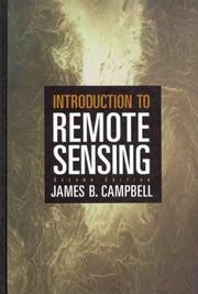
The gentler of the two standard texts, and the better first book: strong on image interpretation, on the history of the sensor systems and on why the discipline developed as it did. Assumes essentially no mathematics beyond secondary school. Now co-authored with Randolph Wynne; the record we link is an earlier printing, and later editions are substantially updated on modern sensors.
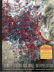
Lillesand, Kiefer and Chipman is the other standard course text and the more comprehensive: photogrammetry, thermal, radar, lidar and digital analysis all covered properly. Assumes basic trigonometry and algebra and introduces the physics as needed. Read it second — Campbell tells you what the field is, Lillesand is the one you keep on the desk. The catalogue record carries an early edition date; buy the most recent edition available.
The physics that makes the numbers mean something
IntermediateBe able to derive rather than recite the sensing chain: source radiance, atmospheric transmission and scattering, surface interaction, sensor response, digital number — and understand why radiometric and geometric correction are not optional preprocessing but the step that turns pixels into measurements.
▸ Study plan for this stage
Pace: Ten to twelve weeks for 956 pages, and this is where the mathematical prerequisites bind. Assumed: multivariable calculus, comfort with wave physics and electromagnetic theory, blackbody radiation, and enough Fourier analysis to follow a transform argument. Rees's Physical Principles of Remote Sensi
- The sensing chain end to end: source radiance, atmospheric transmission on the downward path, surface interaction, atmospheric transmission upward, sensor spectral response, quantisation to a digital number — and the fact that every step is invertible only approximately.
- Radiometric quantities and their units, which are the commonest source of confusion in the field: radiant flux, irradiance, radiance, reflectance, emissivity, and what is per unit solid angle and what is not.
- Blackbody radiation, the Planck function, Wien's displacement law and the Stefan-Boltzmann law, and why they determine which spectral region is useful for measuring temperature.
- Atmospheric interaction: Rayleigh and Mie scattering, absorption by water vapour, ozone, carbon dioxide and other gases, and the atmospheric windows that dictate where sensor bands are placed.
- Why atmospheric correction is not optional preprocessing. Top-of-atmosphere radiance is not a surface property, and any multitemporal comparison of uncorrected data is comparing atmospheres as much as surfaces.
- Surface interaction models: specular against diffuse reflection, the bidirectional reflectance distribution function, and why the same surface returns different radiance to different viewing geometries.
- Geometric correction as a physical problem rather than a warping exercise: platform ephemeris, attitude, sensor geometry and terrain relief each contribute a displacement with its own model.
- The sensor's own physics from Elachi: detector response, noise sources, signal-to-noise ratio, and how the instrument's limits propagate into the uncertainty of any derived product.
- Write out the sensing chain as an equation from surface reflectance to digital number, naming every term you have to know or estimate.
- Distinguish radiance from irradiance and from reflectance, with units. Which of the three is a property of the surface alone?
- Derive the peak emission wavelength for a surface at 300 K and explain why thermal sensors sit where they do.
- Explain why Rayleigh scattering makes the blue band the noisiest and what that implies for atmospheric correction.
- What is the BRDF, and what error do you incur by assuming a Lambertian surface? When is that assumption acceptable?
- List every contribution to geometric distortion in a spaceborne image and say what data each correction requires.
- Derive the Planck function's consequences yourself: compute spectral radiance at several temperatures and plot the curves. The plot explains the entire thermal band placement.
- Work a full radiometric correction on a real scene by hand for a single pixel: digital number to top-of-atmosphere radiance to top-of-atmosphere reflectance to surface reflectance, stating every assumption. Doing this once is worth reading three chapters.
- Compute an atmospheric transmission spectrum from tabulated absorption data and mark the windows. Then check your windows against the band placements in the mission table you built in stage one.
- Take a derivation in Rees and one in Elachi covering the same topic and compare what each assumes of the reader. The comparison tells you which book to reach for later.
Next up: With calibrated physical measurements rather than pixel values, the next stage is about extracting information from them algorithmically.

The best single treatment of the underlying physics at a level a competent undergraduate can follow: electromagnetic theory, radiometry, atmospheric interaction, and the physics of each sensor type. Requires calculus and comfort with wave physics; the mathematics is worked rather than asserted, which is exactly what this stage needs.

Elachi and van Zyl is the harder and more complete treatment, from JPL, and the standard graduate text. It covers wave propagation, interaction mechanisms, orbital mechanics and every sensor family including radar interferometry. Assumes electromagnetics at the level of a physics or electrical-engineering degree — noticeably tougher than Rees, and the reference you will still be using years later.
Digital image processing and classification
BeginnerImplement and reason about the core algorithms: histogram operations and filtering, principal components and other transforms, maximum-likelihood and supervised classification, unsupervised clustering, accuracy assessment with a confusion matrix and kappa, and change detection.
▸ Study plan for this stage
Pace: Twelve to fourteen weeks for 1,691 pages, the longest stage on the path. Assumed: linear algebra including eigen-decomposition, probability and statistics at undergraduate level including multivariate normal distributions and Bayes's theorem, Fourier analysis for the third book, and scripting in Pyt
- The preprocessing chain in the order it must be done, and why radiometric correction precedes geometric resampling — resampling mixes pixel values, so any calculation on physical units belongs before it.
- Histogram operations, contrast enhancement and spatial filtering in both domains, with the convolution-multiplication relationship that connects them.
- Principal components as an eigen-decomposition of the band covariance matrix: what the components mean physically, why the leading ones concentrate the variance, and where the method misleads.
- Maximum-likelihood classification derived rather than recited: the multivariate normal assumption, the class covariance matrices, and the training-sample requirement that follows from having to estimate them. That assumption is the crux — it is what makes the method tractable and what breaks on hype
- Unsupervised clustering with k-means and ISODATA, and the honest limitation that clusters are spectral rather than semantic and must be labelled by someone who knows the ground.
- Accuracy assessment done properly: an independent sample, the confusion matrix, producer's and user's accuracy, overall accuracy, kappa and its well-known criticisms, and the fact that a map without a stated accuracy is not a result.
- Change detection methods and the reason most of them fail: differences in illumination, atmosphere, phenology and registration produce apparent change that has nothing to do with the surface.
- The image-formation model from Schowengerdt: the point spread function, sampling, aliasing and the resampling kernels, and how each produces artefacts that look like data.
- Why must radiometric correction precede geometric resampling? What goes wrong in the other order?
- Derive the maximum-likelihood decision rule from Bayes's theorem, stating every assumption. How many training pixels per class do you need, and why does that number depend on band count?
- What do principal components mean physically for a multispectral scene? Give a case where the leading component is not the most useful one.
- Design an accuracy assessment for a five-class land-cover map: sampling scheme, sample size, and what independence requires.
- Give three sources of apparent change in a two-date comparison that are not surface change, and say how each is controlled.
- What is aliasing in an imaging system, and what does it look like in a final product?
- Implement principal components yourself from the covariance matrix, without using a library function, and compare your output to the library's. The exercise is to see the eigenvectors as band weights rather than as a black box.
- Write a maximum-likelihood classifier from the decision rule and run it on a real scene, then compare it to a library implementation and account for every difference.
- Produce a full accuracy assessment with an independent sample and a confusion matrix, and report producer's and user's accuracy per class. Then write a paragraph on which class failed and why, using the spectral signatures from stage one.
- Take a scene deliberately misregistered by one pixel and run a change detection on it. The result is the argument for why registration accuracy is stated in fractions of a pixel.
- Work one Schowengerdt frequency-domain example completely and identify the same artefact in real data you have processed.
Next up: Everything so far has assumed optical multispectral data, and the next stage takes on the two sensor families where those intuitions actively mislead.

The standard applied text on processing Earth-observation imagery specifically: preprocessing, enhancement, classification, accuracy assessment. Jensen explains the methods with the practitioner's questions in mind rather than the mathematician's, which makes it the right first book of this stage. Requires statistics and comfort with matrices.

The rigorous treatment of the same material: Bayesian classification derived properly, feature reduction, spectral transforms, support vector machines and neural approaches in later editions. Requires linear algebra and probability at a real level. This is the book that turns you from someone who runs a classifier into someone who can say why it failed.
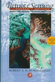
The signal-processing view, and the strongest of the three on the sensor and image-formation models — point spread functions, resampling, the frequency domain, image fusion. Assumes Fourier analysis. Read it third: it explains artefacts the other two books teach you to work around. Catalogued with commas in place of the colon.
The specialist sensor families
BeginnerWork with data that is not optical multispectral: understand radar backscatter, polarimetry and interferometric phase, and the very different statistics of a hyperspectral cube with hundreds of correlated bands.
▸ Study plan for this stage
Pace: Twelve weeks for 1,371 pages, and the prerequisites step up again. Assumed: everything from stage two, plus signal processing, complex analysis and complex-valued arithmetic for the radar books, and linear algebra with detection and estimation theory for the hyperspectral one. Woodhouse's Introducti
- Why radar intuitions differ from optical ones: the sensor supplies its own illumination at a side-looking geometry, so brightness encodes roughness, geometry and dielectric properties rather than reflectance — expressed through the surface, volume and double-bounce backscatter mechanisms, and how ea
- SAR geometry and its distinctive distortions: slant range against ground range, foreshortening, layover and radar shadow, none of which have an optical analogue.
- Aperture synthesis: how a long synthetic aperture is constructed from the platform's motion and the returned phase history, which is the reason azimuth resolution is independent of range.
- Speckle as a coherent-imaging phenomenon rather than noise in the usual sense, its multiplicative statistics, and why multilooking trades resolution for radiometric stability.
- Polarimetry: what the scattering matrix contains, what the polarisation combinations tell you about scattering mechanism, and the decomposition theorems built on that.
- Interferometric phase: coherence, the interferogram, phase unwrapping, and the distinction between topographic and differential interferometry for measuring ground deformation.
- The hyperspectral problem stated correctly: hundreds of narrow contiguous bands are highly correlated, the covariance matrix is ill-conditioned, and classical multivariate classifiers estimated per class break down — which is why detection theory replaces classification as the frame.
- Spectral mixture analysis, endmembers and abundance estimation, and the matched-filter and anomaly-detection formulations that follow from treating the problem as signal detection in coloured noise.
- Explain layover and foreshortening geometrically. Why does neither occur in a nadir-viewing optical image?
- Describe the three main backscatter mechanisms and predict the appearance of a flooded forest, a calm lake and a city block in an L-band image.
- How does aperture synthesis achieve fine azimuth resolution? Give the argument in terms of Doppler history.
- Walk through an InSAR deformation measurement from two acquisitions to a displacement map, naming every step that can fail.
- Why does maximum-likelihood classification break down on a hyperspectral cube? Give the statistical reason, not the computational one.
- State the matched-filter detector for a known target spectrum in coloured noise and say what has to be estimated to use it.
- Take a Sentinel-1 scene over terrain you know and identify layover, shadow and foreshortening by eye. Then confirm each against the topography.
- Compute a multilook average at several look numbers and plot the resulting speckle statistics. The plot is the resolution-against-radiometry tradeoff made concrete.
- Produce an interferogram from a Sentinel-1 pair and attempt phase unwrapping. Where it fails, work out whether the cause is decorrelation, gradient or noise.
- Run spectral unmixing on a hyperspectral cube with endmembers you select yourself, then with automatically extracted ones, and account for the difference in abundances.
- Implement a matched-filter detector and test it on a cube with a known target. Then degrade the covariance estimate deliberately and watch the false-alarm rate move.
Next up: You now understand every major data type on its own terms, which leaves the question of doing all of it at scale on real problems.
The most humane introduction to radar in print, and it genuinely is an introduction — Woodhouse builds the wave physics up carefully before reaching scattering and imaging radar. Start here rather than with a SAR monograph; radar defeats people who skip the fundamentals because the intuitions from optical imaging are actively misleading.

Massonnet and Souyris on SAR proper: synthetic aperture formation, speckle, polarimetry and interferometry, from two authors central to the development of InSAR for ground deformation. Assumes signal processing and complex analysis. The step up from Woodhouse, and the book to read before touching Sentinel-1 phase data.

Manolakis, Lockwood and Cooley approach hyperspectral data as a statistical signal-detection problem — spectral mixture analysis, matched filters, anomaly and target detection — which is the correct frame and rarely taught this well. Heavy on linear algebra and detection theory. The most demanding book on the path.
Doing it on real data
BeginnerMove from understanding methods to running them at scale: write the analysis in code, work in a cloud archive rather than downloading scenes, and be able to take a real applied question from data selection through to a defensible map with stated accuracy.
▸ Study plan for this stage
Pace: Ten to twelve weeks, and one of the four books has no recorded page count. Assumed: programming in Python, R or JavaScript, and everything from the previous stages. Canty's Image Analysis, Classification, and Change Detection in Remote Sensing is 508 pages and closes the gap between the algorithms a
- Reproducibility as a technical requirement rather than a virtue: an analysis that exists only as a sequence of clicks in a desktop package cannot be checked, corrected or rerun on new data.
- The cloud-archive model and what it changes — computation moved to the data, whole archives available without download, and the different cost structure and failure modes that come with it.
- The MAD and IR-MAD transformations for change detection, which Canty derives properly: an invariant, statistically grounded alternative to differencing that is robust to the radiometric differences stage three warned about.
- Training-data design as the dominant determinant of classification quality — sample size, spatial autocorrelation between training and validation pixels, and class balance matter more in practice than the choice of classifier.
- The full applied pipeline as Wegmann and colleagues run it: question, data selection, preprocessing, classification or index computation, validation, and a defensible statement of accuracy.
- Vegetation and biodiversity indices as derived products with assumptions attached, including saturation at high biomass and sensitivity to soil background and view geometry.
- Coordinate reference systems, datums and projections, and the fact that a datum mismatch produces a silent offset of tens to hundreds of metres that no processing step will flag.
- Error propagation through a spatial analysis: positional error, classification error and attribute error compounding through overlay operations, which Bolstad treats explicitly and most workflows ignore — and which is why the deliverable standard here is a map with a stated accuracy, an explicit met
- What does the IR-MAD transformation do that image differencing does not, and what makes it invariant?
- Design a training and validation sampling scheme for a supervised classification. How do you avoid spatial autocorrelation between the two sets, and why does it matter?
- What does moving computation to the archive change about how you would answer a continental-scale question? Name two things that become possible and one new failure mode.
- Explain the difference between a datum and a projection, and describe an error that only a datum mismatch would produce.
- Take a vegetation index and state its assumptions and its failure conditions. When would you not use it?
- Trace error through a two-layer overlay analysis. Where does the uncertainty in the final map come from, and in what proportion?
- Implement IR-MAD from Canty's derivation on a real image pair and compare it to simple differencing on the same data. Explain every difference in the results.
- Take one applied question end to end in a cloud environment — a land-cover map, a burned-area extent, a surface-water time series — from data selection to a validated product with a confusion matrix, and publish the script.
- Reproduce one of the Wegmann chapters on your own study area in R. Then write a paragraph on which step took longest, which is almost always data preparation.
- Deliberately misassign a datum on a real dataset and measure the resulting offset. Then find the same error in someone else's published workflow — it is more common than it should be.
- Write the final deliverable for a question you actually care about: the method, the code, the map, and the accuracy statement, with the limitations section written honestly.
Next up: The path ends with a reproducible analysis of real data, which is the only point at which any of the preceding theory has been demonstrated to have been understood.

The book that closes the gap between the algorithms and your own code: Canty derives each method and then implements it, with the change-detection material — particularly the MAD and IR-MAD transformations — better than anywhere else. Later editions use Python and Google Earth Engine. Assumes you can program.

The modern practical workflow, in the platform where most applied remote sensing is now actually done: the full Landsat and Sentinel archives already on the server, analysed with JavaScript or Python instead of downloaded. Tutorial-led and open-access. The fastest route from the theory above to a working analysis.

A worked applied path in R, aimed at people with a domain question rather than an imaging one: pre-processing, land-cover classification, vegetation and biodiversity indices, validation. The best demonstration on this list of what the whole pipeline looks like when it is pointed at a real research problem.

Remote sensing output is almost always consumed inside a GIS, and the errors that ruin projects are usually projection, datum and topology errors rather than classification ones. Bolstad is the clearest text on coordinate systems, data models, spatial analysis and error propagation. Read it in parallel with anything above rather than last if your GIS is weak.