GIS: a reading path to map and analyze spatial data
This curriculum takes a beginner from zero GIS knowledge to professional-level spatial analysis and development across four carefully sequenced stages. It starts by building core geographic intuition and cartographic literacy, then introduces industry-standard tools (QGIS, PostGIS, Python), and finally advances into spatial analysis theory and scalable geo-development — each stage assuming mastery of the one before it.
Foundations: Geography, Maps & Spatial Thinking
BeginnerUnderstand how the real world is represented digitally — coordinate systems, projections, map design principles, and what GIS actually is — before touching any software.
▸ Study plan for this stage
Pace: 6–8 weeks, ~25–35 pages/day (alternating between both books; start with Monmonier for 2 weeks, then Bolstad for 4–6 weeks)
- Map projections and distortions: why no flat map can perfectly represent a sphere, and how different projections preserve different properties (area, shape, distance, direction)
- Coordinate systems (geographic vs. projected): latitude/longitude, UTM, and how to choose the right system for your data and region
- How maps are inherently subjective: classification schemes, color choices, scale, and generalization all encode human decisions and can mislead or clarify
- Spatial data representation: how the real world is abstracted into raster (grid) and vector (points, lines, polygons) data models in GIS
- Map design principles: visual hierarchy, symbolization, legends, and how to communicate spatial information clearly and honestly
- The purpose and workflow of GIS: data collection, storage, analysis, and visualization as a system for understanding spatial relationships
- Scale and generalization: how detail changes with zoom level and why different scales reveal different patterns
- Accuracy, precision, and uncertainty in spatial data: understanding that all maps contain errors and how to assess data quality
- What are the main types of map projections (conformal, equal-area, equidistant) and what does each preserve? Give an example of when you'd use each.
- Explain the difference between geographic coordinates (lat/long) and projected coordinates (e.g., UTM). Why would you project data before analysis?
- How can a map be technically accurate yet still misleading? Provide three examples from Monmonier of how design choices shape interpretation.
- What are raster and vector data models, and what are the trade-offs between them in terms of storage, analysis, and representation?
- Describe the basic GIS workflow: how does data move from the real world through collection, storage, and analysis to a final map product?
- What role does scale and generalization play in map-making, and how does it affect what spatial patterns are visible or hidden?
- Take a familiar region (your city or country) and find 3–4 maps of it in different projections (e.g., Mercator, Albers, Robinson). Sketch or print them and annotate the distortions you observe—where is area exaggerated? Where are shapes warped?
- Create a simple map of your local area showing two different phenomena (e.g., parks and bus stops). Make one version that emphasizes parks and another that emphasizes transit; document how your color, size, and symbol choices changed the story.
- Collect a dataset of 10–15 real-world locations (addresses, landmarks, GPS coordinates). Convert them to at least two different coordinate systems (lat/long and a projected system like UTM) and calculate distances using both; compare results and explain the differences.
- Read a news article or advertisement that includes a map. Identify three design choices (scale, projection, color, classification) and explain how each choice influences the message or could mislead a casual reader.
- Sketch a simple raster grid (5×5) and a vector representation of the same landscape (e.g., a lake, forest, road). Compare file size, precision, and ease of measuring distance or area in each model.
- Design a choropleth map (color-coded regions) of a dataset you choose (e.g., population density, temperature, election results). Experiment with 2–3 different classification schemes (equal interval, quantile, natural breaks) and write a short reflection on how each changes the visual story.
Next up: This stage establishes the conceptual and visual foundations—understanding how the world is abstracted into data and how to read maps critically—which is essential before learning to create and manipulate spatial data in GIS software in the next stage.
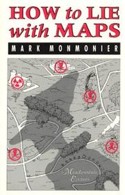
A short, engaging primer on how maps distort reality; builds critical spatial literacy and projection intuition that every GIS user needs from day one.

The most comprehensive beginner-to-intermediate GIS textbook available; covers coordinate systems, data models, spatial analysis, and cartography in a single coherent arc — read it cover-to-cover as your conceptual backbone.
Hands-On Mapping with QGIS
BeginnerBecome productive in QGIS: load, style, and query vector and raster data, perform basic spatial operations, and produce publication-quality maps.
▸ Study plan for this stage
Pace: 8–10 weeks, ~40–50 pages/day (alternating between reading and hands-on practice)
- QGIS interface navigation: toolbars, panels, layer management, and project organization
- Loading and managing vector data (shapefiles, GeoJSON, PostGIS) and raster data (GeoTIFF, satellite imagery) in QGIS
- Styling vector layers: symbology, color ramps, classification schemes, and label placement for clarity and visual hierarchy
- Styling raster layers: band combinations, transparency, and color mapping for effective visualization
- Querying and filtering data using attribute tables, expressions, and spatial queries to extract meaningful information
- Basic spatial operations: buffering, intersecting, dissolving, and spatial joins to answer geographic questions
- Map composition and design: adding titles, legends, scale bars, north arrows, and text annotations for publication-ready output
- Exporting maps in multiple formats (PDF, PNG, SVG) with appropriate resolution and metadata
- How do you load vector and raster data into QGIS, and what are the key differences in how you manage each data type?
- What are the main styling techniques for vector layers, and how do you choose between different classification methods (equal interval, quantile, natural breaks)?
- How do you use the attribute table and expressions to query and filter geographic data in QGIS?
- What are the steps to perform a basic spatial operation (e.g., buffer, intersect, spatial join), and when would you use each?
- How do you compose a publication-quality map, and what elements (legend, scale bar, title, north arrow) are essential for clarity?
- What export formats and settings should you use to produce maps suitable for different media (print, web, presentation)?
- Load a shapefile of administrative boundaries and a raster satellite image into QGIS; practice zooming, panning, and toggling layer visibility
- Style a vector layer using graduated colors based on a numeric attribute (e.g., population density); experiment with different color ramps and class breaks
- Create a second styled layer using categorical symbols (e.g., land-use types); adjust symbol sizes and transparency for visual hierarchy
- Use the attribute table to filter features by a specific criterion (e.g., show only cities with population > 100,000); practice sorting and selecting records
- Write an expression in QGIS to identify features meeting multiple conditions (e.g., roads longer than 10 km AND in a specific region)
- Perform a buffer operation on a point layer (e.g., create 5 km buffers around cities) and export the result as a new shapefile
- Execute a spatial join to count how many points (e.g., schools) fall within each polygon (e.g., district); verify results in the attribute table
- Compose a final map with a real-world dataset: add title, legend, scale bar, north arrow, and source attribution; export as PDF and PNG at publication quality
Next up: Mastery of QGIS fundamentals—data loading, styling, querying, and basic spatial operations—prepares you to tackle advanced spatial analysis, geoprocessing workflows, and custom scripting to solve complex geographic problems.

Written by a core QGIS contributor, this book teaches cartographic best practices directly inside QGIS — a natural first hands-on step after understanding projections and data models.

A step-by-step project-based guide that covers the full QGIS workflow from data import to geoprocessing; read after Map Design to solidify tool fluency with real datasets.
Spatial Databases & Python Geo-Development
IntermediateStore, query, and manipulate spatial data programmatically using PostGIS and Python's geospatial stack (Shapely, Fiona, GeoPandas, Rasterio).
▸ Study plan for this stage
Pace: 12–14 weeks, ~40–50 pages/day (mix of reading and hands-on coding)
- PostGIS architecture: geometry types, spatial indexes, and query optimization for large datasets
- SQL for spatial operations: ST_Distance, ST_Intersects, ST_Buffer, ST_Union, and spatial joins
- Python geospatial libraries: Shapely for geometric operations, Fiona for vector I/O, and GeoPandas for dataframe-based spatial analysis
- Rasterio workflow: reading, writing, and processing raster data (bands, CRS, resampling, windowed reads)
- Coordinate reference systems (CRS) and transformations: understanding EPSG codes and reprojecting data
- Geoprocessing workflows: combining vector and raster operations, automating spatial tasks, and handling large datasets
- Database design for spatial data: schema design, indexing strategies, and connecting Python to PostGIS
- Performance optimization: spatial indexes, query planning, and efficient data loading/processing
- How do you design a PostGIS schema for a real-world spatial dataset, and what indexing strategies improve query performance?
- What is the difference between geometry and geography types in PostGIS, and when should you use each?
- How do you use Shapely to perform geometric operations (buffering, intersection, union) and why is this useful in geoprocessing workflows?
- How do you read vector data with Fiona, transform it with GeoPandas, and write results back to a file or database?
- What are the key steps for reading, processing, and writing raster data with Rasterio, including handling multiple bands and CRS transformations?
- How do you connect a Python script to a PostGIS database, execute spatial queries, and retrieve results into a GeoPandas GeoDataFrame?
- Create a PostGIS database schema for a city planning dataset (buildings, roads, parks); add spatial indexes and write 5 spatial queries (intersection, distance, containment, union, buffer)
- Load a shapefile with Fiona, apply 3 geometric transformations using Shapely (buffer, simplify, convex hull), and write the results to a new shapefile
- Use GeoPandas to read multiple vector datasets, perform a spatial join, calculate statistics by region, and visualize the results with a map
- Write a Python script that reads a multi-band raster with Rasterio, applies a band math operation (e.g., NDVI calculation), and writes the output to a new GeoTIFF
- Build a geoprocessing pipeline: query a PostGIS table, filter results in Python, buffer features, intersect with a raster, and export the final result
- Reproject a vector dataset and a raster dataset to a different CRS using GeoPandas and Rasterio; verify the transformation and compare coordinate values before/after
Next up: This stage equips you with the ability to store, query, and manipulate spatial data at scale using industry-standard tools; the next stage will build on this foundation to tackle advanced topics like spatial analysis, modeling, and real-world applications (e.g., network analysis, terrain analysis, or machine learning with geospatial data).
The definitive PostGIS reference; teaches spatial SQL, geometry types, indexing, and topology — essential before writing any Python code that talks to a spatial database.

Covers the core Python geo stack (GDAL/OGR, Fiona, Shapely, Rasterio) with practical examples; builds directly on PostGIS knowledge by showing how to move data between Python and spatial databases.

Bridges the gap to modern data-science workflows with GeoPandas, Folium, and visualization libraries — read last in this stage to integrate everything into reproducible geo-analysis pipelines.
Advanced Spatial Analysis & GIS Theory
ExpertApply rigorous spatial statistics, network analysis, and geographic data science methods; understand the theoretical underpinnings well enough to design original spatial research or production GIS systems.
▸ Study plan for this stage
Pace: 8–10 weeks, ~40–50 pages/day with code-along sessions; allocate 2–3 days per chapter for hands-on implementation
- Exploratory Spatial Data Analysis (ESDA) and visualization techniques for detecting spatial patterns and anomalies
- Spatial autocorrelation measures (Moran's I, Geary's C, Local Indicators of Spatial Association) and their interpretation
- Spatial weights matrices: construction, row-standardization, and their role in defining spatial neighborhoods
- Spatial regression models (OLS, spatial lag, spatial error) and diagnostics for spatial dependence
- Point pattern analysis: intensity estimation, K-functions, and clustering detection methods
- Network analysis in geographic contexts: shortest paths, centrality measures, and accessibility metrics
- Geostatistics and interpolation: kriging methods, variograms, and uncertainty quantification
- Geographic data science workflow: from raw spatial data to reproducible analysis pipelines in Python
- How do you construct and interpret a spatial weights matrix, and why is row-standardization important in spatial analysis?
- What is Moran's I, how do you calculate it, and what does a Moran's I scatterplot reveal about spatial autocorrelation?
- When should you use spatial lag vs. spatial error models, and how do you diagnose spatial dependence in OLS residuals?
- How do you perform point pattern analysis to distinguish between random, clustered, and dispersed spatial distributions?
- What is kriging, how does it differ from simple interpolation, and how do you construct and interpret a variogram?
- How do you apply network analysis to measure accessibility and centrality in geographic systems, and what are the practical implications?
- Build spatial weights matrices (queen, rook, k-nearest neighbors, distance-based) for a real dataset and compare their properties
- Compute Moran's I and Local Indicators of Spatial Association (LISA) on a geographic dataset; create Moran's I scatterplots and cluster maps
- Fit OLS, spatial lag, and spatial error models to a geographic dataset; run Lagrange multiplier tests and compare model diagnostics
- Perform point pattern analysis on a point dataset: estimate intensity, compute K-functions, and test for clustering using Monte Carlo simulation
- Construct a variogram for a continuous spatial variable, fit a theoretical model, and perform kriging interpolation with uncertainty bands
- Conduct network analysis on a transportation or street network: calculate centrality measures, shortest paths, and accessibility metrics
Next up: This stage equips you with the statistical rigor and Python implementation skills to move into specialized domains—whether designing custom GIS production systems, conducting advanced spatial research, or applying machine learning to geographic data—by grounding theory in reproducible code and real-world datasets.
A methodical, tool-agnostic treatment of spatial pattern analysis, density, and proximity — provides the analytical vocabulary needed before tackling statistical spatial methods.

An open, rigorous textbook combining PySAL, spatial autocorrelation, clustering, and regression in Python; the capstone of this curriculum, synthesizing all prior coding and theory skills.
Discussion
Keep reading
Paths that share books, cover the same subject, or open a related topic.