Best Books on High-Performance and Scientific Computing, in Reading Order
High-performance computing is two disciplines wearing one name: making a machine go fast, and making a numerical answer be right. This path starts with computing as a scientific instrument and the node-level performance engineering that decides most real speedups, moves through MPI and OpenMP parallelism, then builds the numerical foundations — linear algebra, conditioning, stability — before finishing with accelerators and the floating-point questions that decide whether a fast answer is worth having.
Computing as a scientific instrument
IntermediateWrite correct, reasonably fast serial scientific code, and understand the memory hierarchy and node architecture well enough to know where the time is actually going.
▸ Study plan for this stage
Pace: Three to four months. Computational Physics is 561 pages and is a working textbook — plan on one chapter a week with the exercises actually coded, roughly two months. Hager and Wellein is 356 pages and much denser per page; six weeks at 10 to 15 pages a session, benchmarking as you go. Read Newman f
- Newman's central working habit: solve a problem you know the answer to before solving one you do not. Every numerical method in his book is introduced against a physical problem with a checkable result, and this is how you learn to distinguish a bug from a physical effect
- The memory hierarchy as the actual determinant of performance — registers, L1, L2, L3, main memory — with roughly two orders of magnitude between the fastest and slowest, and the fact that a modern core spends most of its time waiting
- Memory bound versus compute bound, and the arithmetic intensity that distinguishes them: flops per byte moved. Most scientific kernels have low arithmetic intensity, which is why they run far below peak and why buying more flops does not help
- The roofline model, which is the single most useful diagram in the field: peak performance and memory bandwidth as two ceilings, and a kernel's arithmetic intensity placing it under one or the other. Hager and Wellein build it carefully and it should become how you think
- Spatial and temporal locality, cache lines, and why loop order in a nested loop over a matrix can change runtime by an order of magnitude with no change to the arithmetic performed
- SIMD vectorisation and what prevents it: aliasing, dependencies, non-unit stride, branching. Getting a loop to vectorise is usually about removing an obstacle rather than adding an instruction
- NUMA and first-touch placement, which is where most people's first multi-socket disappointment comes from: memory is allocated near the thread that first writes it, so initialisation code determines the performance of computation code
- The measurement discipline underneath all of it: a timing without a baseline, a repeat count and a check on the answer is not a result
- What is arithmetic intensity, and how do you compute it for a simple stencil or a dense matrix multiply? Which of the two is memory bound?
- Draw a roofline for a machine you have access to. Where does a vector triad land, and where does a dense GEMM land?
- Why does traversing a matrix in the wrong index order cost so much more, when the same number of floating-point operations is performed?
- What is false sharing, at what granularity does it occur, and why does it appear only in threaded code?
- Explain first-touch NUMA placement. Why can an initialisation loop determine the scalability of a completely different loop?
- Newman insists on validating before optimising. Give a concrete case where optimising first would have hidden a physics error
- Implement a naive matrix multiply, then a loop-reordered one, then a blocked one, and measure all three against a tuned BLAS on your machine. Plot the results. This single experiment teaches more about the memory hierarchy than any chapter about it.
- Run the STREAM benchmark on your machine, record the achieved bandwidth, and use it to draw the memory ceiling of your roofline. Then measure a real kernel and place it on the plot.
- Take one of Newman's physics problems — the simple pendulum or a diffusion equation is ideal — and verify your solution against an analytical result before you time anything. Then profile it and predict where the time goes before you look.
- Take a loop the compiler refuses to vectorise, find out why from the compiler's optimisation report, and remove the obstacle. Compilers will tell you if you ask, and learning to read that report is a permanent skill.
- Time the same code ten times and report the distribution rather than the minimum. Understanding your own measurement noise is a prerequisite for every claim you will make in the remaining stages.
Next up: Most of a real speedup comes from the node-level work you have just done, which is exactly why you should attempt parallelism only now — with a profiled, validated serial baseline to scale against.

The most approachable route in: real physical problems solved computationally, with the numerical methods introduced as they become necessary. It establishes the habit of validating a result before optimising it.

The best single HPC text and the intellectual core of this path: cache behaviour, the roofline model, data access optimisation and why most codes are memory bound rather than compute bound. Almost everyone's first real speedup comes from this book, not from parallelism.
Parallel programming
IntermediateDecompose a problem across processes and threads, and write, debug and scale a real MPI plus OpenMP application on a cluster.
▸ Study plan for this stage
Pace: Five to six months. An Introduction to Parallel Programming is 450 pages and should be worked rather than read — two months with the exercises coded. Using MPI is 337 pages and is a practical reference; six weeks reading and writing distributed code simultaneously. Using OpenMP is 384 pages, another
- Domain decomposition versus task decomposition, and the halo or ghost cell exchange pattern that dominates practical scientific MPI codes
- Amdahl's law and Gustafson's law as the two ways to ask a scaling question — fixed problem size versus fixed time — and why strong and weak scaling plots answer different questions and are routinely confused
- MPI's point-to-point semantics in Gropp: the difference between blocking, buffered, synchronous and non-blocking sends, and the deadlock that a naive exchange between neighbours produces
- Communicators and derived datatypes, which are the two MPI features that separate people who use MPI from people who know it — a derived datatype lets you send a strided subarray without packing it by hand
- Non-blocking communication and computation-communication overlap, which is the main structural optimisation available in a distributed code and the reason to prefer Isend and Irecv as a default habit
- OpenMP data scoping — shared, private, firstprivate, reduction — which is where nearly all OpenMP bugs live, and the fact that a wrongly scoped variable produces a wrong answer rather than a crash
- False sharing and the loop-scheduling choices (static, dynamic, guided) that determine load balance, plus the affinity settings that decide whether your threads stay where you put them
- Hybrid MPI plus OpenMP as the standard production shape — one rank per socket or NUMA domain, threads within it — and the reasons it beats either model alone on modern nodes
- Take a 2D stencil problem and write out its domain decomposition, including exactly which halo cells each rank must exchange with which neighbour
- Why does a ring exchange written with blocking sends deadlock, and give three distinct fixes
- State Amdahl's law and compute the maximum speedup for a code that is 95% parallel. Then explain why weak scaling can look good for the same code
- What is an MPI derived datatype and when is it better than packing a buffer manually?
- Which OpenMP data-scoping mistake produces a race that only appears at high thread counts, and how would you detect it?
- Why does a hybrid MPI plus OpenMP code usually outperform pure MPI on a modern many-core node? Give the memory and communication reasons separately
- Parallelise the validated serial code from stage one with OpenMP, then with MPI, and produce both strong and weak scaling plots out to the largest core count you can get. Label which law each plot is testing.
- Deliberately write the deadlocking ring exchange, confirm it hangs, then fix it three ways — reordering, sendrecv, and non-blocking. Watching it hang once is worth more than reading about it.
- Implement a halo exchange with a derived datatype for the strided dimension rather than a manual pack, and measure both. The performance difference is often small and the code difference is large.
- Restructure one loop to overlap communication with computation using non-blocking calls, and measure whether the overlap actually happened. It frequently does not, and finding out why is the real lesson.
- Introduce a false-sharing bug on purpose by having threads update adjacent array elements, measure the slowdown, then pad the structure and measure again. The factor is usually shocking.
- Run the same code under a correctness tool for races and a profiler for imbalance. Distinguishing a race from a load imbalance from a communication bottleneck by their signatures is the debugging skill this stage is for.
Next up: You can now make a code run fast on many cores, which raises the question the next stage answers: whether the algorithm you are running fast is the right one, and whether its answer is trustworthy.

The standard teaching text, covering MPI, Pthreads, OpenMP and CUDA with the same worked problems in each. Read it first because the side-by-side comparison is what teaches you which model fits a given problem.
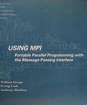
Written by the people who built MPICH, and still the authoritative practical guide to point-to-point and collective communication, communicators and derived datatypes. This is the reference you keep open while writing distributed code.

The shared-memory counterpart: worksharing, data scoping, synchronisation and the false-sharing traps that silently destroy scaling. Read after Gropp, since production HPC codes are almost always hybrid.
Numerical foundations
BeginnerChoose the right algorithm for a linear system, eigenproblem or quadrature, and reason about conditioning, error propagation and cost rather than trusting a library call.
▸ Study plan for this stage
Pace: Eight to twelve months, and this is the deepest stage in the path. Read Heath first as the survey — 448 pages over two to three months with the exercises. Trefethen and Bau's Numerical Linear Algebra is 374 pages in forty short lectures and is the highest-leverage book here; do roughly one lecture p
- Conditioning versus stability, which is the distinction the whole stage turns on: conditioning is a property of the problem, stability is a property of the algorithm, and a stable algorithm applied to an ill-conditioned problem still gives a bad answer. Heath is relentless about this and he is right
- The condition number of a matrix and what it predicts — roughly how many digits you lose — and why estimating it is cheap enough that there is no excuse for not knowing it
- Backward error analysis as the standard framing: rather than asking how wrong the answer is, ask what nearby problem the computed answer solves exactly. This reframing is Wilkinson's and it makes the whole subject tractable
- Why you never form a matrix inverse to solve a linear system, and why the normal equations square the condition number and should be avoided for least squares in favour of QR
- The SVD as the most informative decomposition — rank, conditioning, least squares, low-rank approximation all fall out of it — and the practical habit of reaching for it when you do not yet know what is wrong
- Krylov subspace methods (conjugate gradient, GMRES) and preconditioning, which is where large sparse problems are actually solved and where the preconditioner rather than the solver determines whether you converge
- Golub and Van Loan's blocked formulations and the BLAS level 1, 2 and 3 distinction: the same operation count restructured to reuse data in cache, which is exactly the stage-one memory argument reappearing inside the algorithms
- Quadrature, interpolation and ODE integration in Heath, including stiffness and why an explicit method on a stiff problem takes absurdly small steps for stability reasons that have nothing to do with accuracy
- Define conditioning and stability and give an example of an ill-conditioned problem solved by a stable algorithm. What can you say about the answer?
- Why are the normal equations a bad way to solve least squares, and what does QR do differently? Quantify the difference in terms of condition number
- What does the SVD tell you about a matrix that an LU factorisation does not? List at least four things
- Why does conjugate gradient converge quickly for some matrices and slowly for others, and what is a preconditioner actually doing?
- What is stiffness in an ODE system, and why does it force implicit methods? Give the stability rather than accuracy argument
- Explain the BLAS level 1, 2, 3 distinction in terms of arithmetic intensity from stage one. Why does level 3 dominate performance?
- Solve the same least squares problem three ways — normal equations, QR, and SVD — on a deliberately ill-conditioned design matrix, and compare the answers against a known solution. The divergence between the three is the most persuasive argument in numerical analysis.
- Work through Trefethen and Bau's lectures on the SVD and then compute the SVD of a small matrix by hand. It is tedious once and permanently clarifying.
- Take a sparse system from a real problem and solve it with conjugate gradient, first unpreconditioned and then with a simple preconditioner. Plot the residual history. The preconditioner is usually worth more than every optimisation from stages one and two combined.
- Implement blocked matrix multiplication following Golub and Van Loan's formulation and compare against your stage-one blocked version. Notice that the numerical analysts and the performance engineers arrived at the same structure for different reasons.
- Look up a routine you use routinely in Numerical Recipes and read the section on when it fails. Then check whether your own code guards against those cases. Most does not.
- Integrate a stiff ODE system with an explicit method and watch the step size collapse, then repeat with an implicit method. Report the total function evaluations for both.
Next up: With the algorithms and their error behaviour understood, the last stage moves to the hardware where most performance now lives and asks how much of a fast answer you are entitled to believe.

The clearest survey of numerical methods for a computational scientist — linear systems, least squares, eigenvalues, interpolation, ODEs, PDEs — with consistent attention to conditioning and stability throughout.
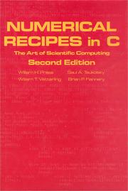
The working practitioner's shelf reference: an algorithm, an explanation of when it fails, and code, for essentially every routine you will need. Best used alongside Heath rather than as a substitute for him.

Forty short lectures that make QR, SVD, conditioning and iterative methods genuinely intuitive. Since dense and sparse linear algebra dominate scientific computing time, this is the highest-leverage theory on the path.

The definitive reference behind every serious linear algebra library, including the blocked and parallel formulations that make these algorithms fast on real hardware. Take it after Trefethen, whose intuition it presupposes.
Accelerators and the limits of precision
BeginnerPort a kernel to a GPU and reason about its performance in terms of occupancy and memory bandwidth, while knowing precisely how much of the resulting answer you are entitled to believe.
▸ Study plan for this stage
Pace: Six to nine months. Structured Parallel Programming is 432 pages and takes about two months — read it before touching CUDA, because it gives you the vocabulary to describe what you are about to write. Programming Massively Parallel Processors is 576 pages and needs three months with a GPU in front o
- The pattern vocabulary from McCool, Reinders and Robison — map, reduce, scan, stencil, fork-join, pipeline, gather and scatter — which lets you state a parallel design before choosing an API, and makes porting between OpenMP, CUDA and anything newer a translation rather than a rewrite
- The CUDA execution model in Kirk and Hwu: grids, blocks, warps and threads, with the warp as the true unit of execution and divergence within a warp as the first thing to check when a kernel underperforms
- The GPU memory hierarchy — global, shared, constant, registers — and coalescing, which is the same spatial-locality argument from stage one restated for a machine where the penalty for getting it wrong is much larger
- Occupancy, and the important correction to the naive view: maximum occupancy is not the goal, sufficient occupancy to hide memory latency is. Register pressure and shared memory use trade against it
- Host-device transfer as the usual real bottleneck. A kernel that is ten times faster than the CPU version and moves data across PCIe every iteration is slower than the code it replaced
- Higham's central result set: the standard model of floating-point arithmetic, error bounds for summation, inner products, and matrix factorisations, and the fact that these bounds are worst case and usually pessimistic in practice
- Why summation order matters and what to do about it — compensated summation and pairwise summation — which is directly relevant because every parallel reduction reorders the sum
- Reduced and mixed precision, which is where the machine learning era has pushed HPC: half precision has a very small exponent range and few significand bits, and iterative refinement is the classic technique for getting a high-precision answer out of low-precision factorisation. Higham is the author
- Express a stencil computation, a histogram and a sort in the pattern vocabulary. Which of the three is a scan in disguise?
- What is warp divergence, what causes it, and how would you detect it in a profiler?
- Explain memory coalescing on a GPU and give a code change that turns an uncoalesced access into a coalesced one
- State the standard model of floating-point arithmetic. What is the error bound for summing n numbers naively, and how does pairwise summation improve it?
- Your MPI reduction gives a slightly different answer on 64 ranks than on 32. Is this a bug? Explain precisely
- When is it legitimate to factor in half precision and refine in double, and what determines whether the refinement converges?
- Port the kernel you have carried through the whole path to CUDA, and place it on a GPU roofline. Compare the fraction of achievable bandwidth you reach on the GPU against what you reached on the CPU in stage one.
- Implement a parallel reduction three ways — naive, tree, and with compensated summation — and compare both the runtime and the answer against a high-precision reference. This exercise is the entire thesis of the final stage in one experiment.
- Deliberately write an uncoalesced access pattern, measure it, then fix it and measure again. Then do the same for a divergent branch. Two experiments, two permanent instincts.
- Time a GPU kernel including and excluding the host-device transfer and report both numbers. Reporting only the second is the most common dishonesty in GPU performance claims and you should know exactly how large the gap is.
- Implement iterative refinement: factor in a lower precision, refine in a higher one, and plot the residual per iteration. Then find the condition number at which it stops converging.
- Write a final one-page performance and accuracy report for your kernel — baseline, optimisations applied, speedup, scaling behaviour, and the error bound on the result. Producing that page for a real code is what this entire path was for.
Next up: This is the end of the path: you can profile and optimise a node, scale across a cluster, choose and analyse the algorithm, use accelerators, and state how much of the answer to believe.

Teaches the parallel patterns — map, reduce, scan, fork-join, pipeline — as a portable design vocabulary above any one API. The right framing before touching GPU-specific code.

The standard GPU computing text: the CUDA execution model, memory hierarchy, coalescing, occupancy and a set of worked parallel algorithm patterns. Where node-level performance work now mostly happens.

The definitive treatment of floating-point error analysis, and a deliberately sobering close. Parallelism and reduced precision both change the answer you compute, and this is the book that tells you by how much.
Discussion
Keep reading
Paths that share books, cover the same subject, or open a related topic.