Bioinformatics: books to analyze genomes and biological data
This curriculum takes an intermediate learner from the core concepts of sequence analysis and genomics through the algorithmic and statistical machinery that powers modern bioinformatics, finishing with the computational and data-science skills needed to work with large biological datasets. Each stage builds directly on the vocabulary and intuition established in the previous one, so reading within and across stages in order is essential.
Foundations of Bioinformatics
IntermediateEstablish a solid working vocabulary in sequence alignment, genomics, and the core problems bioinformatics solves, while getting comfortable with the biological context behind the algorithms.
▸ Study plan for this stage
Pace: 8–10 weeks, ~40–50 pages/day (mix of reading and algorithm walkthroughs). Week 1–3: Compeau's foundational chapters on sequence alignment and genome assembly; Week 4–6: Durbin's HMMs and probabilistic models; Week 7–8: Durbin's advanced topics (phylogenetics, gene finding); Week 9–10: Integration an
- Sequence alignment algorithms (dynamic programming, Smith-Waterman, Needleman-Wunsch) and their biological interpretation
- Scoring matrices (PAM, BLOSUM) and gap penalties as biological assumptions
- Hidden Markov Models (HMMs) as a unifying framework for sequence analysis and profile building
- Genome assembly problem: how to reconstruct genomes from short reads and the role of de Bruijn graphs
- Probabilistic inference in biology: using Bayes' theorem to infer evolutionary relationships and functional elements
- Multiple sequence alignment and its role in detecting homology and inferring function
- Gene finding and annotation: combining signal detection with probabilistic models
- The central problems of bioinformatics: homology detection, functional annotation, and evolutionary inference
- Explain the difference between global and local sequence alignment, and describe when you would use Smith-Waterman vs. Needleman-Wunsch in a real biological scenario.
- What biological assumptions are encoded in a BLOSUM62 matrix, and how would you choose a different scoring matrix for comparing distantly related proteins?
- Describe how a Hidden Markov Model can be used to represent a protein family, and explain what the emission and transition probabilities represent biologically.
- Walk through the de Bruijn graph approach to genome assembly: how do overlapping reads become nodes/edges, and what does finding an Eulerian path accomplish?
- Given a multiple sequence alignment, how would you use it to build a profile HMM, and what biological insights does the resulting model capture?
- Explain how Bayes' theorem is applied in gene finding: what are the prior and likelihood terms, and what biological knowledge do they encode?
- Implement the Needleman-Wunsch algorithm from scratch (pseudocode or code) for global alignment; test it on two short protein sequences and trace the dynamic programming table by hand.
- Manually compute a Smith-Waterman local alignment between two sequences using a BLOSUM62 matrix; compare your result to a BLAST search on the same sequences.
- Download a protein family from Pfam or InterPro; build a multiple sequence alignment (using Clustal or similar), then sketch out the structure of an HMM that would model that family.
- Implement or simulate a simple de Bruijn graph construction from a set of short reads; identify an Eulerian path and reconstruct the original sequence.
- Use an HMM-based tool (like HMMER) to search a sequence database with a profile HMM; interpret the E-values and bit scores in terms of statistical significance.
- Analyze a real gene annotation (e.g., from NCBI or Ensembl) and reverse-engineer the probabilistic model that might have been used to predict exon/intron boundaries.
Next up: Mastery of sequence alignment, HMMs, and probabilistic inference provides the algorithmic and statistical foundation needed to tackle specialized topics like structural prediction, RNA analysis, and systems-level bioinformatics in the next stage.

A problem-driven introduction that builds algorithmic intuition from scratch using real biological questions — ideal for an intermediate learner who needs both the biology and the computation framed together from the start.
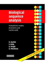
The canonical text on probabilistic models (HMMs, profile models) for sequences; reading it after Compeau ensures the underlying biology and alignment concepts are already in place before tackling probabilistic formalism.
Algorithms and Data Structures for Genomics
IntermediateUnderstand the key algorithms — suffix arrays, BWT, graph-based assembly, read mapping — that power modern genomics pipelines, and be able to reason about their correctness and efficiency.
▸ Study plan for this stage
Pace: 8–10 weeks, ~40–50 pages/day (mix of dense algorithmic content and code walkthroughs). Allocate 4–5 weeks to Jones, then 4–5 weeks to Mäkinen. Plan 2–3 days per major algorithm for deep study and implementation.
- Suffix arrays and suffix trees: construction, querying, and their role in pattern matching and sequence alignment
- Burrows-Wheeler Transform (BWT): compression, reversibility, and application to read indexing and alignment
- Graph-based genome assembly: de Bruijn graphs, overlap graphs, and resolving ambiguity in assembly
- Read mapping and short-read alignment: seed-and-extend paradigm, hash tables, and handling mismatches/gaps
- Time and space complexity analysis: understanding O(n log n) vs O(n) construction and query costs in genomic contexts
- Practical trade-offs: memory efficiency, construction speed, and query speed in real genomics pipelines
- Correctness reasoning: why these algorithms produce correct results and how to verify them on test cases
- How do suffix arrays enable fast pattern matching in genomic sequences, and what are the advantages over naive string search?
- Explain the Burrows-Wheeler Transform: how it works, why it is reversible, and how it supports efficient read alignment.
- What is a de Bruijn graph, and how does it resolve the overlap-graph assembly problem for short reads?
- Describe the seed-and-extend paradigm for read mapping: what role do seeds play, and how do you handle mismatches?
- Compare the time and space complexity of suffix array construction vs. suffix tree construction. When would you choose one over the other?
- How do modern genomics pipelines (e.g., BWA, Bowtie) leverage BWT and FM-indexing for efficient alignment of millions of reads?
- Implement a suffix array construction algorithm (e.g., naive O(n² log n) or optimized O(n log n)) and test it on a small DNA sequence.
- Build a pattern-matching tool using a suffix array: given a reference genome and a query sequence, find all occurrences and report positions.
- Implement the Burrows-Wheeler Transform and its inverse on a genomic sequence; verify reversibility.
- Construct a de Bruijn graph from a set of short reads (k-mers) and trace a path through it to reconstruct a contig.
- Write a seed-and-extend read mapper: hash k-mer seeds from reads, find matches in a reference, and extend with dynamic programming to refine alignments.
- Benchmark suffix array vs. hash table lookup for read mapping on a real dataset (e.g., 1000 reads against a 1 Mbp reference); document memory and runtime trade-offs.
Next up: Mastery of these core algorithms provides the computational foundation needed to understand how real-world genomics tools are engineered and optimized, and prepares you to explore variant calling, sequence assembly quality metrics, and advanced indexing strategies in the next stage.
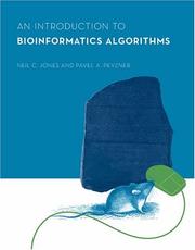
Provides rigorous algorithmic treatment of dynamic programming, graph algorithms, and combinatorics as applied to biology, bridging the gap between the conceptual stage and deeper algorithmic study.

Covers modern compressed data structures, the Burrows-Wheeler transform, and read alignment at a depth matched to someone who has already internalized basic sequence algorithms — the natural next step.
Statistics and Machine Learning for Genomics
IntermediateApply statistical inference, hypothesis testing, and machine learning methods to genomic data, understanding both the theory and the practical pitfalls (multiple testing, batch effects, high dimensionality).
▸ Study plan for this stage
Pace: 8–10 weeks, ~40–50 pages/day, with 2–3 days per week dedicated to computational exercises and problem sets
- Probability distributions and their role in modeling biological variation (normal, Poisson, binomial, negative binomial)
- Hypothesis testing framework: null distributions, p-values, Type I/II errors, and power analysis in genomic contexts
- Multiple testing correction (Bonferroni, FDR, q-values) and why naive p-values fail with thousands of genomic features
- Exploratory data analysis and visualization techniques for high-dimensional genomic data (PCA, heatmaps, MA plots)
- Linear models and ANOVA for comparing groups in RNA-seq and microarray studies, including design matrices and contrasts
- Batch effects, confounding variables, and practical strategies for detection and correction (ComBat, SVA, blocking)
- Regularization and dimensionality reduction: ridge regression, LASSO, and principal component regression for genomic prediction
- Resampling methods (permutation tests, bootstrap) for robust inference when parametric assumptions are violated
- Why is the negative binomial distribution more appropriate than the Poisson for RNA-seq count data, and what does overdispersion tell us about biological variation?
- Explain the multiple testing problem in genomics: why does a naive p-value threshold of 0.05 fail when testing 20,000 genes, and how do FDR-controlling procedures address this?
- How do you design and interpret a linear model for RNA-seq differential expression analysis, including the role of design matrices, contrasts, and model assumptions?
- What are batch effects, how do they manifest in genomic data, and what are the trade-offs between detection methods and correction approaches?
- When would you use regularization (ridge, LASSO) over ordinary least squares regression in a genomic prediction task, and what does the regularization parameter control?
- Describe a complete workflow for analyzing a microarray or RNA-seq experiment: from exploratory analysis through multiple testing correction to biological interpretation
- Reproduce the probability distribution examples from Holmes (normal, Poisson, negative binomial) using R; fit these distributions to real RNA-seq or microarray count data and assess goodness-of-fit
- Conduct a simulation study demonstrating Type I error inflation under multiple testing; compare raw p-values, Bonferroni, and FDR correction on synthetic genomic data with known signal
- Perform PCA on a real genomic dataset (e.g., from GEO or Bioconductor); interpret the principal components, identify potential batch effects or confounders, and visualize with biplots and scree plots
- Fit linear models to RNA-seq or microarray data using design matrices; test multiple contrasts (e.g., treatment vs. control, interaction effects) and validate model assumptions (residual plots, Q-Q plots)
- Detect and correct batch effects in a multi-batch genomic dataset using both visualization (PCA before/after) and statistical methods (e.g., ComBat or SVA from Bioconductor); compare the impact on downstream differential expression results
- Implement a regularized regression model (ridge or LASSO) for genomic prediction; use cross-validation to select the regularization parameter and compare performance to ordinary least squares on held-out data
Next up: This stage equips you with the statistical and machine learning foundations needed to handle the complexity, high dimensionality, and multiple-testing challenges inherent in genomic data, preparing you to advance to specialized topics such as variant calling, genome-wide association studies (GWAS), or single-cell RNA-seq analysis where these principles are applied to specific biological questions.

A hands-on, R-based treatment of the statistical concepts most relevant to biological data — distributions, testing, clustering, and visualization — written specifically for biologists and bioinformaticians.
Provides the rigorous probabilistic and statistical foundations (Markov chains, likelihood, Bayesian inference) that underpin the methods introduced in Holmes, deepening theoretical understanding.
Programming and Data Analysis in Practice
IntermediateTranslate algorithmic and statistical knowledge into reproducible, scalable code using Python and R, and learn the standard libraries and workflows used in real bioinformatics research.
▸ Study plan for this stage
Pace: 8–10 weeks, ~40–50 pages/day (mix of reading and hands-on coding)
- Python fundamentals for biological data: strings, lists, dictionaries, and file I/O for parsing FASTA/FASTQ files
- Writing reusable, modular code with functions and object-oriented programming principles tailored to bioinformatics workflows
- Data manipulation and exploratory analysis using command-line tools, shell scripting, and version control (Git)
- Working with tabular biological data: parsing, filtering, and transforming genomic datasets using Python and R
- Reproducible research practices: documentation, testing, and organizing bioinformatics projects for scalability
- Standard bioinformatics file formats (FASTA, FASTQ, SAM/BAM, GFF, VCF) and how to parse them programmatically
- Introduction to R for statistical analysis and visualization of biological data
- Debugging, profiling, and optimizing code for performance on large genomic datasets
- How do you parse and manipulate FASTA and FASTQ files using Python, and what are the key differences between these formats?
- What are the principles of writing modular, reusable code in Python, and how do functions and classes improve bioinformatics workflows?
- How do you use the command line and shell scripting to automate repetitive bioinformatics tasks, and why is this essential for reproducibility?
- What is version control (Git), and why is it critical for collaborative and reproducible bioinformatics research?
- How do you read, filter, and transform tabular genomic data (e.g., variant calls, gene annotations) using Python or R?
- What are best practices for organizing a bioinformatics project, documenting code, and testing for correctness?
- Write a Python script to parse a FASTA file, extract sequences of a specific length, and output them to a new file; refactor it into reusable functions
- Create a command-line tool in Python that filters FASTQ files by quality score and read length; test it on real sequencing data
- Set up a Git repository for a bioinformatics project, make commits with meaningful messages, and practice branching and merging workflows
- Parse a VCF (variant call format) file using Python; filter variants by quality and allele frequency, then output results to a new VCF
- Write R code to load a CSV of gene expression data, perform basic statistical summaries, create visualizations (boxplots, scatter plots), and save results
- Build a small bioinformatics pipeline (e.g., read quality control → alignment filtering → variant annotation) using shell scripts and Python; document each step
Next up: This stage equips you with the practical coding and data-handling skills to implement the algorithmic and statistical concepts you'll encounter in advanced topics like sequence alignment, phylogenetics, and machine learning applications in genomics.

A focused, biology-motivated Python primer that gets the reader writing file parsers, sequence processors, and data scripts quickly — essential before tackling larger frameworks.

Covers the full practical stack — Unix, Python, R, reproducible pipelines, and working with large genomic files — and is best read after Python fundamentals are in place so the reader can immediately apply every tool shown.
Advanced Topics: Networks, Single-Cell, and Systems Biology
ExpertEngage with cutting-edge areas of bioinformatics including gene regulatory networks, single-cell RNA-seq analysis, and systems-level thinking, synthesizing everything from prior stages.
▸ Study plan for this stage
Pace: 8–10 weeks, ~25–35 pages/day, with 2–3 days per week dedicated to computational exercises and network visualization projects
- Gene regulatory networks (GRNs): motifs, feedback loops, and dynamic behavior as fundamental building blocks of biological systems
- Systems-level thinking: emergence, robustness, and modularity in biological networks and how they enable complexity from simple components
- Single-cell RNA-seq data: handling sparsity, dimensionality reduction, clustering, and trajectory inference to resolve cellular heterogeneity
- Computational genome analysis: sequence alignment algorithms, hidden Markov models, and statistical inference for genomic pattern discovery
- Integration of multi-omics data: connecting transcriptomics, proteomics, and metabolomics within systems biology frameworks
- Network inference and reconstruction: reverse-engineering biological networks from high-dimensional data using correlation, mutual information, and causal methods
- Temporal dynamics and bifurcations: understanding how biological systems transition between states and respond to perturbations
- Scalability and computational challenges: managing large-scale genomic and single-cell datasets with efficient algorithms and tools
- What are the three main types of gene regulatory network motifs described by Alon, and why are they considered fundamental building blocks? How do they contribute to biological robustness and information processing?
- How does systems biology differ from reductionist approaches in molecular biology, and what does it mean for a biological system to exhibit emergence?
- Describe the workflow for analyzing single-cell RNA-seq data: from raw counts to cell-type identification and trajectory inference. What are the key computational challenges at each step?
- Explain the role of hidden Markov models in computational genome analysis. How are they used for sequence annotation and what assumptions underlie their application?
- How would you design a study to infer a gene regulatory network from single-cell RNA-seq data? What are the limitations of correlation-based versus causal inference methods?
- What is the relationship between network topology (e.g., scale-free properties, modularity) and biological function? Provide examples from Alon's work.
- Reconstruct and visualize a simple gene regulatory network motif (e.g., negative feedback, feedforward loop) using Python/R; simulate its dynamics under different parameter regimes and observe bifurcation behavior
- Download a published single-cell RNA-seq dataset (e.g., from GEO or 10x Genomics); perform quality control, normalization, dimensionality reduction (PCA/UMAP), and clustering; compare results across different clustering algorithms
- Implement or use an existing tool (e.g., SCENIC, GRNBoost) to infer a gene regulatory network from single-cell data; validate predicted interactions against known regulatory relationships in a reference database
- Work through Waterman's sequence alignment examples: implement or trace through a dynamic programming algorithm for global/local alignment; calculate alignment scores and interpret statistical significance
- Build a hidden Markov model for a simple genomic annotation task (e.g., CpG island detection); train it on a reference sequence and apply it to predict features in a test genome
- Integrate single-cell transcriptomics with protein abundance data (if available) to construct a multi-omics network; identify hub genes/proteins and their functional roles using pathway enrichment
Next up: This stage synthesizes network inference, single-cell resolution, and computational genomics into a unified systems perspective, preparing you to tackle specialized applications such as disease modeling, drug target discovery, or organism-specific systems biology projects in subsequent stages.

Builds quantitative intuition about biological networks and design principles — a conceptual bridge from sequence-level analysis to systems-level reasoning that rewards readers who already understand genomics.
Integrates probability, statistics, and algorithms in a unified framework for genome-scale problems, serving as a capstone that ties together all prior stages into a coherent advanced perspective.
Discussion
Keep reading
Paths that share books, cover the same subject, or open a related topic.